Introduction
Engineering is about solving problems, given some constraints. My name is Adam, and I'm a software engineer. I write code. Many of my colleagues at Zoo are hardware engineers. They design and build real-world objects. Some people see software and hardware engineering as two different disciplines. After all, software can't be touched or seen. It can't keep the two ends of a bridge together. And hardware -- everything from bridges to buildings to clamps to rockets -- can. Physical and software systems seem very separate. But that's not how I see it. Both coders and Formula 1 car designers are fundamentally engineers. We're both trying to solve difficult problems, with limited resources and various constraints. We're both trying to satisfy some requirement (like function) while minimizing some measurements (like cost or size) and still making the final result comprehensible (to our colleagues, to our users, or to our future self who revisits this project in two years).
Zoo started when Jess, a software engineer, called Jordan, an aerospace engineer, about her struggles with a really complicated CAD model. The two realized they had a lot more in common than they thought. They realized that if software and hardware engineers take the best parts of each other's practices and tools, we could get our jobs done quicker and with less stress. Every day at Zoo, we put bright engineers from all disciplines together and let them learn from each other.
These days, hardware engineers need to use software. The days of hand-drawing all your designs on a drafting table are over. But hardware engineers often find their software frustrating. Software engineers understand -- ranting about how much you hate software is a time-honored tradition among software engineers. The difference is, when software engineers don't like their tools, they know how to take them apart and make new ones. We can find the source code for our software, fork it, and add new features. Or we could even write our own version from scratch, that works exactly how we'd like it to. Unfortunately, when hardware engineers don't like their software, they're stuck. They don't usually know enough programming to edit their engineering software. So they're at the mercy of some software engineer at a different company, who doesn't understand the problem well enough. Our goal at Zoo is to put the software and hardware engineers in the same room, so that when hardware engineers complain about their tool, the software people are listening and can quickly improve it. Experimenting with ideas from both worlds will be the key to modern, 21st century engineering.
KCL is one of the first successes from this hardware-software-engineer collaboration. We hope it will make CAD both easier to understand and more powerful. KCL, or the KittyCAD Language, is a programming language for CAD.
Why a programming language?
Zoo's programmers -- experts in programming languages -- listened to Zoo's aerospace engineers, and concluded that what they needed was... a programming language! Surprise surprise. No, wait, don't run away aerospace engineers! It's not that bad, I promise!
Hardware engineers often shudder when I tell them we're building a programming language for CAD. I understand why! CAD is complicated. Programming is complicated. Simplifying CAD with programming is like solving your rampaging boar problem by introducing rampaging lions to control them. But we really believe in this approach. We've seen first-hand the benefits of code-driven CAD. We know other software has tried to combine them, but we think they started with three fundamental flaws:
- The code has to be fundamental. You can't build a non-code CAD suite and then slap code on afterwards. Otherwise, there'll be gaps between these two halves -- things you can do in code but not in the "normal software", and vice-versa.
- Not everyone will want to code -- and that's OK. If you don't want to learn KCL, you don't have to! You can still use a traditional mouse-based, point-and-click workflow if you're more comfortable there. Every time you click a button, Zoo Design Studio is actually generating KCL under the hood. You've been writing KCL without knowing it! Or more accurately, telling the computer to write the KCL for you. If you decide to learn KCL later, you can open up your existing models and view the KCL.
- Reusing existing languages. JavaScript, C, Python etc are all great languages. But they were designed for software engineering, and the problems that software engineers solve. KCL is designed for engineering real world objects, not software. So it makes different choices. Existing languages require you to learn a bunch of little details that matter a lot to programmers, but aren't really important to mechanical engineers. KCL doesn't have any of those. Instead, it has built-in features that match how mechanical engineers think.
Learning to code takes work. Why bother learning KCL if you can just use the point-and-click UI instead? There's a few reasons.
Firstly, KCL lets you read the fundamental model underlying your designs. In normal CAD software, if you want to understand your model, you have to spin it around in the UI, look at different parts, maybe hide or show various faces that would block your view of its internals. This is because you never really access the model directly. Instead, you view a rendering of the model. Feature trees help, but they only show a subset of the information connecting your model. KCL lets you directly read the exact same code that our CAD suite is executing. If you want to know why a hole has a certain diameter, you can just go to the line of code which defines that hole, and see where it gets its length. Is it a direct measurement, handwritten like length = 2mm? Is it a parameter from a parametric design? Is it the result of a calculation, like length = totalHeight * 0.3? Code makes it easy to see exactly where your measurements come from.
Secondly, KCL is the interface between human and computer. Programming languages aren't really built for computers. Computers use binary instructions like 1101010101010100000011. The first computers had to be programmed in binary, and coders would look up each instruction carefully in a huge reference manual to find which 0s and 1s each instruction needed. This was obviously very tedious, so programming languages were invented instead. Both humans and machines can read code like let x = y + 3. The human knows what it means, and the computer knows how to execute it.
Lastly, KCL is the interface between humans and other humans. Let's say you're collaborating on a CAD model with a coworker. They send you the latest revision of some part, and you open it up. What's changed? Impossible to tell. You'd have to open up the old revision and glance back-and-forth between the two to find the difference. This is much easier when your model is stored as code! You can easily see the exact lines of code that changed -- green for new lines added, red for old lines removed, yellow for changes. And your coworker can leave comments in the code, so that anyone reading it understands exactly what has changed. As a bonus, this works even for solo engineers. If you want to see how your model has changed since last year, you can open up last year's file and run the same line-by-line visual comparison.
By learning KCL, you're developing a skill that can open up massive improvements to your design and engineering skills. It's a new skill, and like all new skills it takes time and practice to develop. But it's worth it. Code-driven CAD can become your superpower and let you simplify your designs and design quicker. I'm excited to guide you on this journey. Let's get started.
Installation
There are two main ways to work with KCL. You can use Zoo Design Studio, our all-in-one application built specifically for KCL designs, or you can use a traditional programming interface with your own text editor. We definitely recommend the Zoo Design Studio.
Zoo Design Studio
You can download Zoo Design Studio, then open it and get started. There's a KCL code pane -- click the Code Editor button on the left edge of the screen. That's it! Get ready to design in KCL.
You'll note that when you write KCL code, the live 3D view updates, showing the model you've defined. And if you use the point-and-click buttons (to draw lines, or to select faces for extruding, or edges for filletting), the corresponding lines of code get highlighted. This two-way communication between the code and visuals is the key reason we think KCL will succeed where other code-CAD solutions failed. It's easy to tell exactly what part of the model your code corresponds to.
Traditional code editing
You can download the Zoo CLI, which lets you execute KCL programs and download some sort of visualization. You can download your KCL models as 3D files or as 2D images. Use zoo kcl --help to learn more.
You can edit KCL in whatever text editor you prefer. If you're using VSCode you can use our VSCode extension. For all other editors, our LSP and Tree-sitter grammar are available. If you're interested in adding support for other editors or developer tools, please let us know! We're happy to work with you for more open-source KCL support.
Contributing to KCL
Our GitHub for Zoo Design Studio has all of our developer tooling and the language runtime. Please take a look there if you'd like to open any bugs or contribute to KCL! This book itself is available on GitHub too. Feel free to open issues or PRs.
Variables
Let's get comfortable with basic KCL first, before we start designing parts. Don't worry, we'll get to real mechanical engineering very soon. For now, let's start with some math.
Here's a simple KCL program. Open up the Zoo Design Studio, make a new project, then open the KCL code panel (on the left). Enter this text in:
width = 1
height = 2
area = width * height
This simple program declares three variables. Variables are little bits of data you can define or calculate. Here we define width and height and assign their value immediately. We write their value right in there, as width = 1 and height = 2. You can see that a variable declaration has the variable's name (e.g. width), then an equals sign (=) and then its value (e.g. 1).
The area variable is very similarly, except instead of defining the exact number, we define it as a calculation. We define it as width * height. We could have defined area as just area = 2, but this way, anyone else who reads the code can understand why the area is 2 -- it's because we're calculating some rectangular area with a width and height.
In this simple case, we can calculate the area in our head. It's going to be 2. But what if you're calculating something more complex? Well, take a look at the Variables panel (on the left).
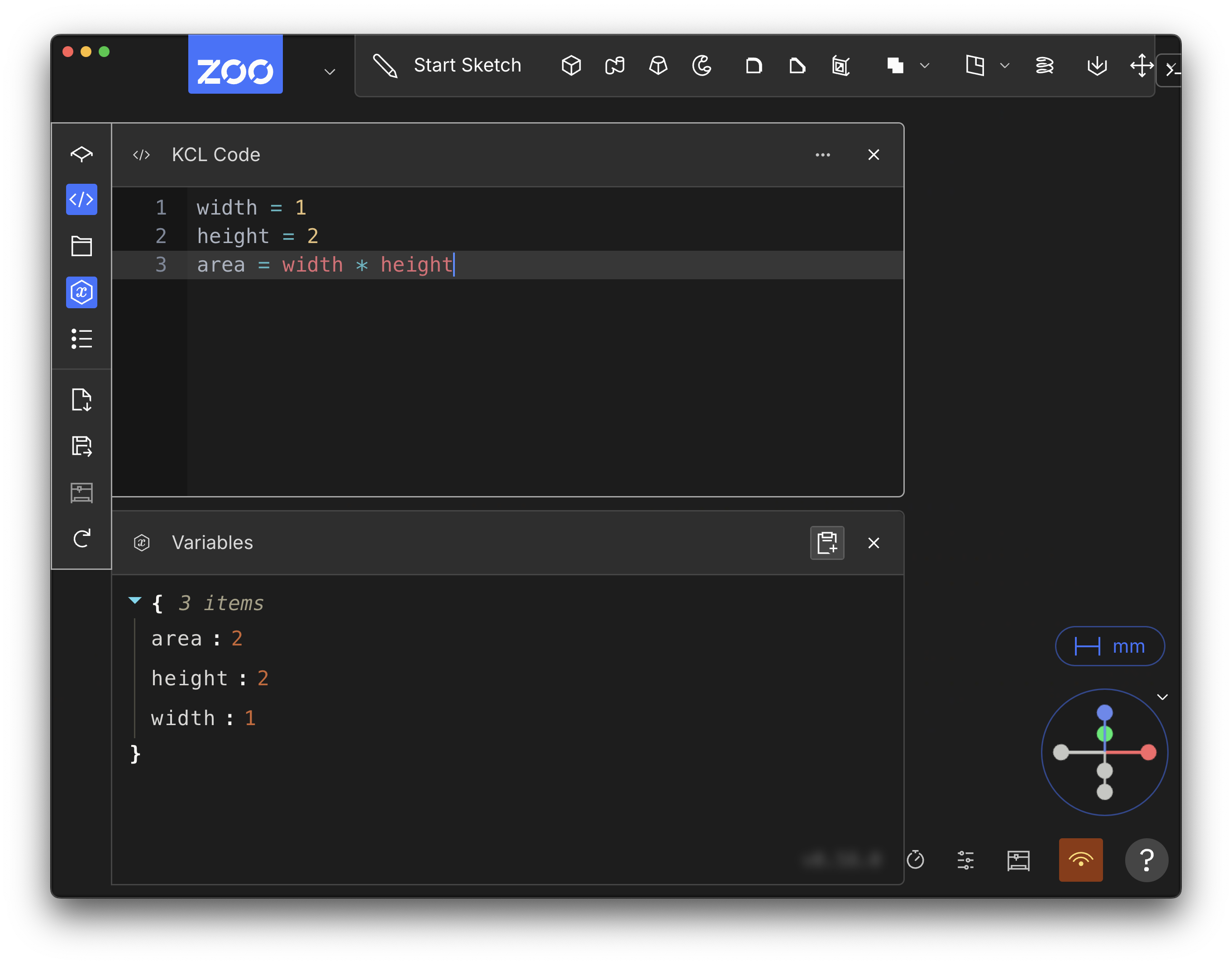
This panel shows every variable and its value. You can look up the value of area here. It's 2, just like we expected. For this simple example it's not necessary to look it up, but for more complicated cases it can be very helpful! This way, you can do all your engineering calculations in KCL. You can treat it like a really advanced calculator, where big equations can be broken into smaller named variables, and their value can be inspected independently.
Note that once you declare a variable, you cannot redeclare it, or change its value.
Basic data types
All the variables in the previous section stored numbers. But KCL can store other types of data too. Let's see some examples. These aren't all the types of data KCL can store, but it's a good starting point. We'll learn more data types later in this book as we get into more specialized features for designing parts.
Number
You just saw how basic numbers work in the example above. Numbers can also be fractional or negative.
Examples
width = 1diameter = 1.5offset = -2.3
Booleans
A boolean value is either true, or false. That's it! Just those two choices. Booleans are useful for changing details of KCL functions, like changing whether a semicircle is drawing clockwise or not.
Examples
clockwise = falseisConstructionGeometry = true
String
A string stores text. "String" is the software-engineering term for text. We probably should have called this just "Text" in KCL, but oh well. You can think of it as "stringing" several letters together to make words. They're not currently used very often in KCL, except to set colours (with the hexadecimal colour codes you might see in Photoshop, Figma or Canva). In the future, you'll be able to use strings to embed text into your models (e.g. for engraving text into your objects).
Examples
textToEngrave = "My Phone"red = "#FF0000"
Collection types
All the previous data types stored basically one piece of data. It might be a number, or text, or a true/false value, but it's basically a single piece of data. KCL variables can also store multiple pieces of data, kept together under a single variable name. Let's see some examples.
Arrays
An array is a list of data, like the four numbers [1, 2, 3, 4] or these three colours ["#ff0000", "#cccc00", "#44ff00"]. These arrays contain other data. We say that arrays contain items. The two previous example arrays had 4 items and 3 items respectively. Sometimes the items of an array are called their elements. The terms "elements" and "items" are synonyms, you can use them interchangeably.
To access the items in an array, you use square brackets and the number item you want. For example, myArray[0] will get the first item from the array, myArray[1] will get the second, and so on. Yes, that's right, the first item is item 0, not item 1! This might be strange for new programmers, but it's how almost every programming language works, so we felt it was important to stick with that convention, so that your KCL code works like similar code in Python, JavaScript, C or other languages.
If you try to access an item beyond what the array contains -- for example, the fifth element of [1, 2] -- you'll get an error and the KCL program will stop.
Arrays can also be defined as a range of values, for example, [1..5] is a shorthand for the array [1, 2, 3, 4, 5]. Note that the range is inclusive at both ends (it includes both the start and end of the range in the array).
Examples
colors = ["#ff0000", "#cccc00", "#44ff00"]red = colors[0]sizes = [33.5, 31.5, 30]smallest = sizes[2]arrayOfArrays = [[1, 2, 3], [1, 4, 6]]firstFiveNumbers = [1..5]
Points
To properly dimension and sketch out your designs, you'll frequently need to select specific points on a plane. In KCL, points can be stored in variables and used just like any other data type. We actually store points as arrays. An array with 2 elements Arrays are really important in KCL, because we use them to represent 2D points on a plane (e.g. the origin [0, 0]) or 3D points in space.
Examples
origin = [0, 0]myPoint = [4, 0, 0]myPointX = myPoint[0]myPointY = myPoint[1]myPointZ = myPoint[2]
Objects
Sometimes, you need to store several pieces of related data together. KCL has objects which contain several fields. Fields have a key, which is always text (a string), and a value, which can be any kind of KCL value. Even another object!
Examples
sphere = { radius = 4, center = [0, 0, 3.2] }wires = { positive = [1, 2], negative = [3, 4], resistance = 0.3 }components = { name = "Flange", holes = { inner = [[0, 0], [1, 0]], outer = [[4, 4]] } }
More info
We used several different operators so far, including + and -, but KCL supports a lot of other operators. You can find a full list in the operator docs.
Calling functions
In the last chapter, we looked at different data types that KCL can store. Now let's look at how to actually use them for more complex calculations. We use KCL functions for nearly everything, including all our mechanical engineering tools, so they're very important.
Data in, data out
Let's look at a really simple function call.
smallest = min([1, 2, 3, 0, 4])
This is a variable declaration, just like the variables we declared in the previous chapter. But the right-hand side -- the value the variable is defined as -- looks different. This is a function call. The function's name is min, as in "minimum".
Functions have inputs and outputs. This function has just one input, an array of numbers. When you call a function, you pass it inputs in between the parentheses/round brackets. Then KCL calculates its output. You can check its output by looking up smallest in the Variables panel. Spoiler: it's 0. Which is, as you'd expect, the minimum value in that array.
If you hover your mouse cursor over the function name min, you'll find some helpful documentation about the function. You can also look up all the possible functions in our standard library documentation. That page shows every function, and if you click it, you can see the function's name, inputs, outputs and some helpful examples of how to use it.
All functions take some data inputs and return an output. The inputs can be variables, just like you used in the previous chapter:
myNumbers = [1, 2, 3, 0, 4]
smallest = min(myNumbers)
A function's inputs are also called its arguments. A function's output is also called its return value.
Here are some other simple functions you can call:
absoluteValue = abs(-3)
roundedUp = ceil(12.5)
shouldBe2 = log10(100)
Labeled arguments
The min function takes just one argument: an array of numbers. But most KCL functions take in multiple arguments. When there's many different arguments, it can be confusing to tell which argument means what. For example, what does this function do?
x = pow(4, 2)
If you mouse over the docs for pow (or look them up at the KCL website) you'll see it's short for power, as in raising a number to some power (like squaring it, or cubing it). But, does pow(4, 2) mean 4 to the power of 2, or 2 to the power of 4? You could look up the docs, but that gets annoying quickly. Instead, KCL uses labels for the parameters. The real pow call looks like this:
x = pow(4, exp = 2)
Now you can tell that 2 is the exponent (i.e. the power), not the base. If a KCL function has multiple arguments, only the first argument can be unlabeled. All the following arguments need a label. Here are some other examples.
oldArray = [1, 2, 3]
newArray = push(oldArray, item = 4)
Here, we make a new array by pushing a new item onto the end of the old array. The old array is the first argument, so it doesn't need a label. The second argument, item, does need a label.
Combining functions
Functions take inputs and produce an output. The real power of functions is: that output can become the input to another function! For example:
x = 2
xSquared = pow(x, exp = 2)
xPow4 = pow(xSquared, exp = 2)
That's a very simple example, but it shows that you can assign the output of a function call to a variable (like xSquared) and then use it as the input to another function. Here's a more realistic example, where we use several functions to calculate the roots x0 and x1 of a quadratic equation.
a = 2
b = 3
c = 1

delta = pow(b, exp = 2) - (4 * a * c)
x0 = ((-b) + sqrt(delta)) / (2 * a)
x1 = ((-b) - sqrt(delta)) / (2 * a)
If you open up the Variables panel, you'll see this gives two roots -0.5 and -1. Combining functions like this lets you break complicated equations into several small, simple steps. Each step can have its own variable, with a sensible name that explains how it's being used.
Comments
This is a good point to introduce comments. When you start writing more complex code, with lots of function calls and variables, it might be hard for your colleagues (or your future self) to understand what you're trying to do. That's why KCL lets you leave comments to anyone reading your code. Let's add some comments to the quadratic equation code above:
// Coefficients that define the quadratic
a = 2
b = 3
c = 1

// The quadratic equation's discriminant
delta = pow(b, exp = 2) - (4 * a * c)

// The two roots of the equation
x0 = ((-b) + sqrt(delta)) / (2 * a)
x1 = ((-b) - sqrt(delta)) / (2 * a)
If you type //, any subsequent text on that line is a comment. It doesn't get executed like the rest of the code! It's just for other humans to read.
The standard library
KCL comes built-in with functions for all sorts of common engineering problems -- functions to calculate equations, sketch 2D shapes, combine and manipulate 3D shapes, etc. The built-in KCL functions are called the standard library, because it's like a big library of code you can always use.
You can create your own functions too, but we'll save that for a future chapter. You can get pretty far just using the built-in KCL functions! We're nearly ready to do some actual CAD work, but we've got to learn one more essential KCL feature first.
Pipeline syntax
When you have repeated function calls wrapping each other, it can become difficult to understand your code. KCL code relies heavily on pipelines to keep code readable. Let's get into the details and learn how to write neater, idiomatic KCL.
The |> operator
In the previous chapter we learned how to call functions: you write the function's name, then give its inputs in parentheses, like this:
x = pow(2, exp = 2)
What if you want to repeatedly call a function, then call another function on that output? Here's an example:
sqrt(sqrt(sqrt(64)))
We find the square root of 64, then pass its output as the input to another square root call. And another. And another. Eventually we've found the eighth root of 64.
This is pretty hard to read! We could make it more readable by breaking it up into single calls and assigning each to its own variable, like this:
x = 64
y = sqrt(x)
z = sqrt(y)
w = sqrt(z)
But then we have to think of meaningful names, and add a lot of variables. Now the Variables pane shows all these intermediate variables like y and z. Sometimes that's helpful, but sometimes it can be distracting.
Passing the output of a function into another function's input is a very common task in KCL code. So, KCL has a nice little feature for simplifying this common pattern. It's called a pipeline. Let's rewrite the above using pipeline syntax:
x = 64
w = sqrt(x)
  |> sqrt(%)
  |> sqrt(%)
What's going on here? Basically, if you call two functions like g(f(x)) you could rewrite it as f(x) |> g(%). Whatever is to the left of the |> gets calculated, then passed into the function on the right of |>. The % symbol basically means "use whatever was to the left of |>". The |> is basically a triangle pointing to the right, showing that the data on the left flows into the function on the right. You can think of it like an assembly line in a factory, moving parts (data) between different machines (functions) using a conveyor belt (the |> symbol).
Let's see another example. If you take a number's square root, and then square it again, it should give you the original number back. Let's test that.
x = 64
xRoot = sqrt(x)
shouldBeX = pow(xRoot, exp = 2)
Let's rewrite this using pipelines:
x = 64
shouldBeX = sqrt(x)
  |> pow(%, exp = 2)
Implicit %
All those %s can be a bit annoying to read. Remember how some KCL functions declare a special unlabeled first argument? If a function uses the special unlabeled argument, then that argument will default to %. Basically, if you use these functions in a pipeline, you can omit the % and KCL will insert the % for you.
In other words, these two programs are equivalent:
x = 8
  |> pow(%, exp = 2)
and
x = 8
  |> pow(exp = 2) // No % needed.
x equals 64 in both these programs.
Let's see another example. We could simplify this program:
x = 64
w = sqrt(x)
  |> sqrt(%)
  |> sqrt(%)
as
x = 64
w = sqrt(x)
  |> sqrt()
  |> sqrt()
Both programs work the exact same -- the first unlabeled argument in sqrt isn't given, so it defaults to %, i.e. the left-hand side of the |> symbol. This makes your code a bit cleaner and easier to read.
With that, you've learned the basics of KCL. You know how to declare data in variables, compute new data by calling functions, and join many functions together (either using pipelines or new variables). We're ready to get into mechanical engineering. In the next chapter we'll start looking at how KCL functions can define geometric shapes for your designs and models.
Sketching 2D shapes
Let's use KCL to sketch some basic 2D shapes. Sketching is a core workflow for mechanical engineers, designers, and hobbyists. You can either sketch fixed geometry, where you manually position your lines, points and curves, or you can use unconstrained geometry, then add constraints later to pin them down into a fixed position. We'll walk through both these options. Let's start with fixed geometry. Then we'll use constraints to think more like an engineer.
Fixed geometry: your first triangle
Let's sketch a really simple triangle. We'll sketch a right-angled triangle, with side lengths 3, 4 and 5.
Just copy this code into the KCL editor:
@settings(defaultLengthUnit = mm, kclVersion = 1.0)

myTriangle = sketch(on = YZ) {
  line(start = [0, 0], end = [0, 3])
  line(start = [0, 3], end = [4, 3])
  line(start = [4, 3], end = [0, 0])
}
When you're done, use the Camera Cube in the corner and select the "Right" face. The camera should swivel around and face your triangle head-on. Your screen should look something like this:
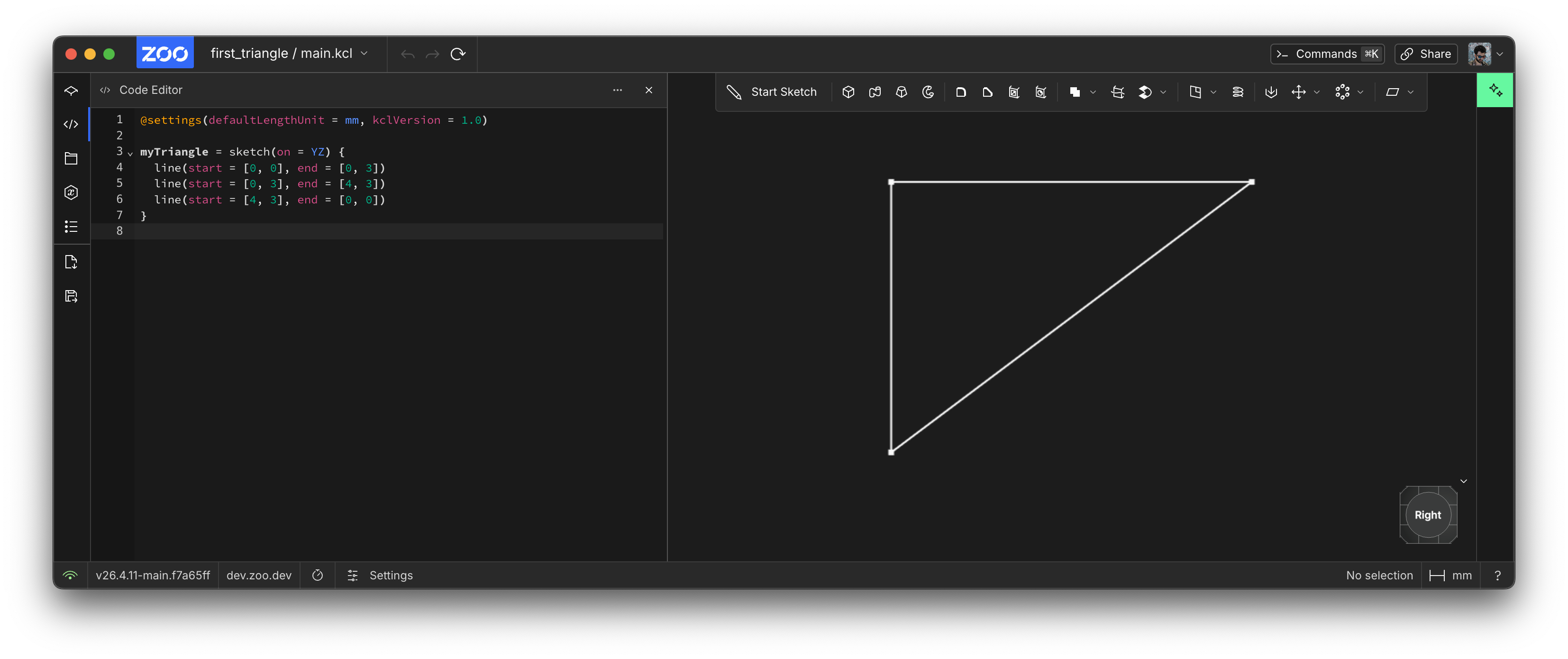
Congratulations, you've sketched your first triangle! Rendering your first triangle is a big deal in graphics programming, and sketching your first triangle is a big deal in KCL. Let's break this code down line-by-line and see what it's actually doing.
1: Set KCL settings
This step is optional, but it's good practice. KCL lets you set a few settings at the top of your file, with @settings(...). Zoo Design Studio will usually set this line for you when you make a new file, and then you can change it later. In @settings(defaultLengthUnit = mm, kclVersion = 1.0), we're choosing two settings:
- Set the default unit to millimeters. This means that when you write a point like
[4, 3]it's treated as 4 millimeters and 3 millimeters. You could write them manually, via[4mm, 3mm]instead. But it's good to set these defaults, so everyone knows that[4, 3]means 4x3 millimeters, not inches or yards or meters. You could replacemmwithcm,m,in,ft, orydinstead. - Set the KCL version to
1.0. This way, in the future, we could add new features in KCL 1.2 without affecting your old code.
2: Choose a plane
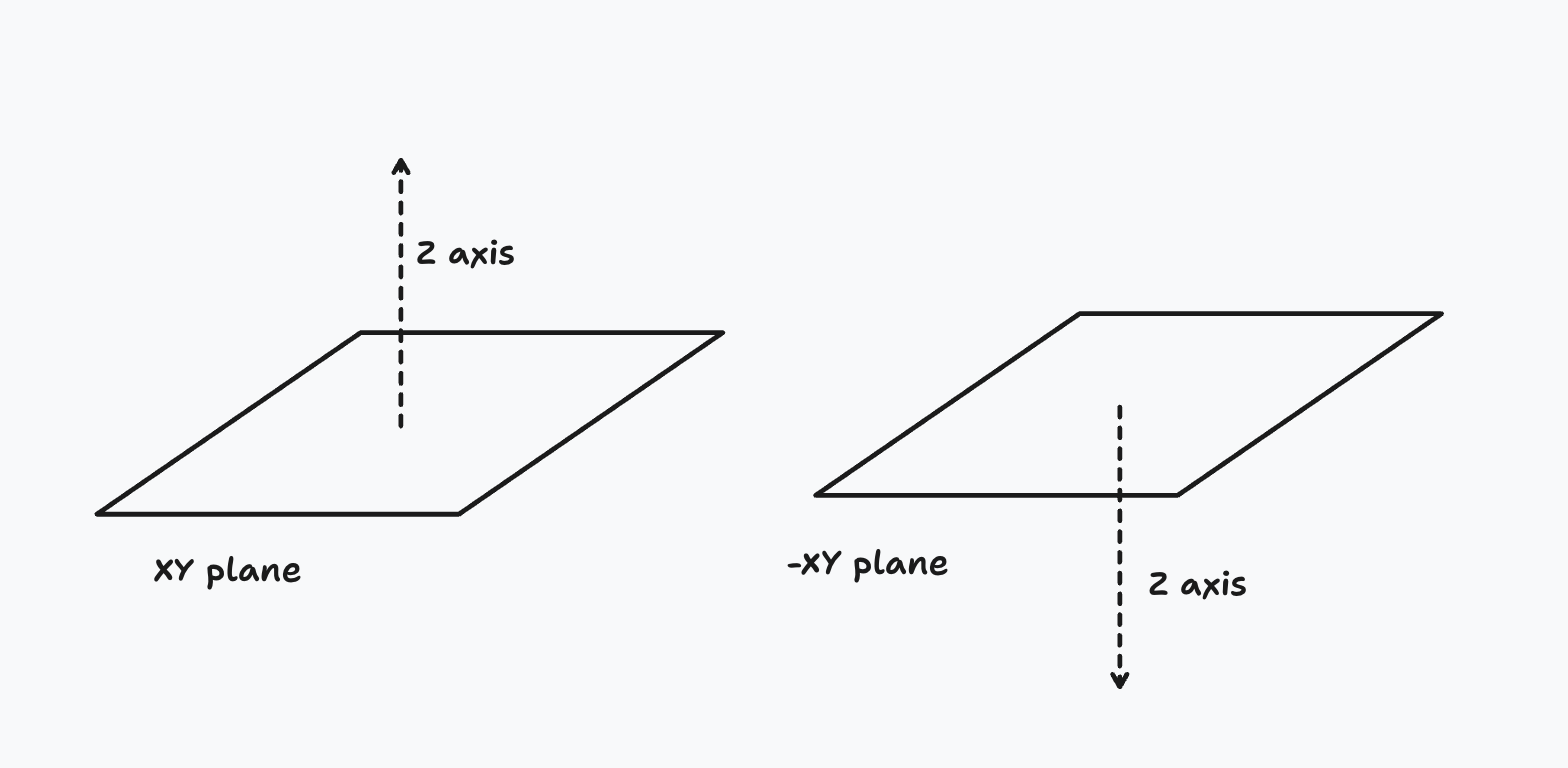
In KCL, there are six basic built-in planes you can use. There's XY, YZ, XZ, and negative versions of each (-XY, -YZ and -XZ). These negative planes are in the exact same place as their matching positive planes, but treat their normal axis (in other words, the axis considered "up") as the opposite direction. For example, XY and -XY share an X and Y axis, but their Z axes are flipped. Extruding "up" in the XY plane and "up" in the -XY plane are opposite directions.
You can use one of these standard planes, or define your own (we'll get to that later). Those six standard planes can be used just like normal variables you define, except they're pre-defined by KCL in its standard library.
You can also sketch on the face of a solid, instead of a plane. But we'll cover that later, in a dedicated chapter on sketch on face.
3: Start a sketch block
Line 3, sketch(on = YZ), is where we actually start sketching. This line declares a sketch block. A sketch block has two parts:
- A list of arguments (enclosed by parentheses
(...)). Right now, there's only one argument:on, where we pass the plane chosen in step 2, e.g.on = YZ. - A sketch block (enclosed by braces,
{...}). The sketch block defines geometry (like lines or arcs), and relationships between them. Our first sketch block will be very simple, with 3 straight lines. We'll build more complex examples later.
4: Add geometry
Sketches contain geometry like lines, arcs, circles and points. In our example sketch, we added three straight lines, each with a start and end. These lines are created by the line function, which takes two parameters: a start and an end. We make a line like this: line(start = [0, 0], end = [0, 3]).
Working with constraints
For simple geometry, like a single triangle, manually positioning the endpoints of lines works just fine. But when you're making more complex shapes, it's hard to choose the positions of every point. Mechanical engineers rarely work out every point's true location in 3D space. Instead, they start with a few pieces of information -- some initial guesses -- and then they add more requirements, letting their CAD suite tweak the geometry to meet these requirements. In other words, they constrain their initial guesses.
Let's start with a goal: sketching a rhombus. There are many ways to define a rhombus, but we'll use this definition: "a parallelogram in which the diagonals are perpendicular". Now, we could use a pen and paper to do some high-school geometry and work out where all 4 points of our rhombus go. That works for this simple example, but it's just not feasible for more complex geometry. Instead, let's just put some initial guesses in, and use KCL's built-in constraint solver to ensure we build a rhombus.
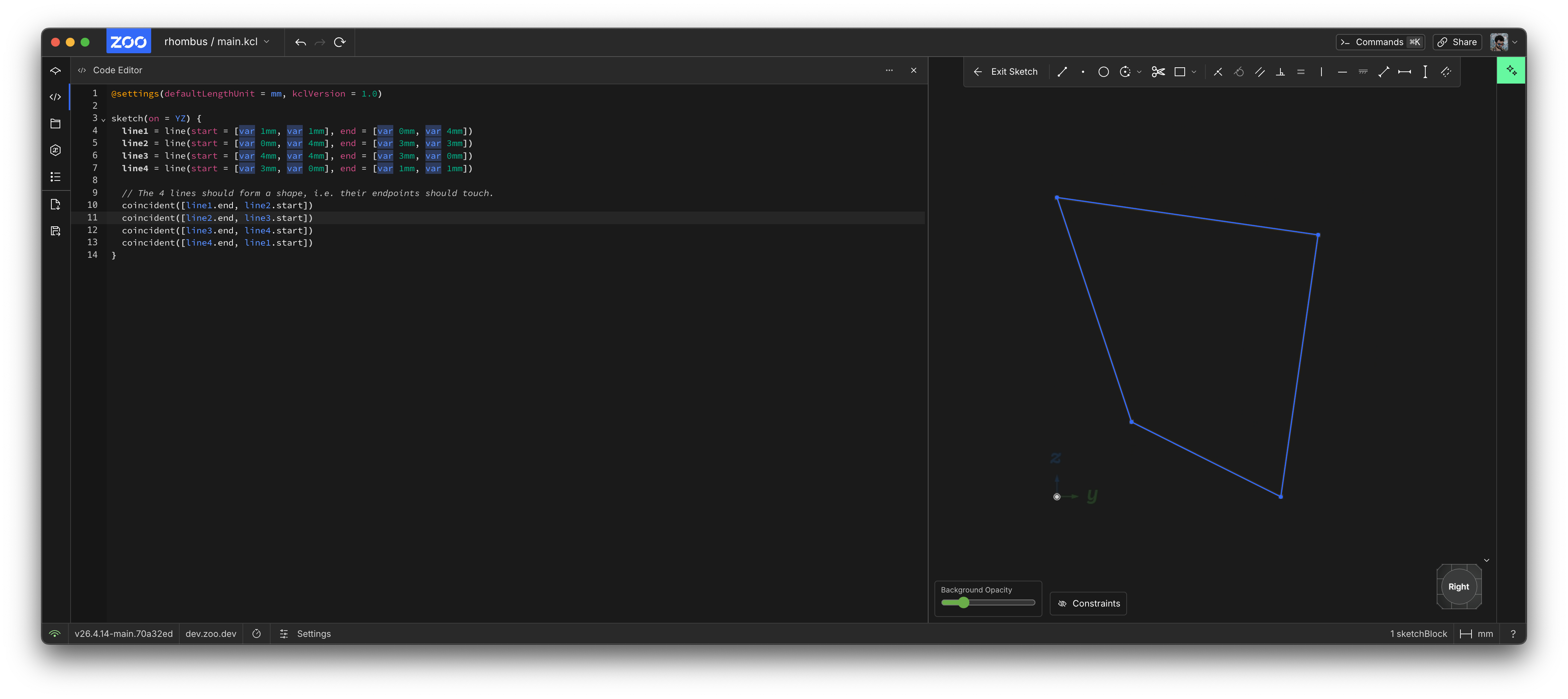
To start, we know our rhombus will have 4 lines. So let's put in some rough guesses.
@settings(defaultLengthUnit = mm, kclVersion = 1.0)

sketch(on = YZ) {
  line1 = line(start = [var 1mm, var 1mm], end = [var 0mm, var 4mm])
  line2 = line(start = [var 0mm, var 4mm], end = [var 3mm, var 3mm])
  line3 = line(start = [var 4mm, var 4mm], end = [var 3mm, var 0mm])
  line4 = line(start = [var 3mm, var 0mm], end = [var 1mm, var 1mm])
}
This looks pretty similar to our earlier triangle example, with two big differences.
First, we're assigning each line to a variable. We've got 4 lines and 4 variables: line1, line2, line3 and line4. This isn't strictly necessary yet -- each line function works just fine on its own, without being assigned to a variable, as you saw in the triangle example earlier. By assigning our geometry to variables, we can give each line a name. We can then refer to line1 or line2 later in your sketch block.
Secondly, we're using the var keyword, for the start and end arguments. This means each line's endpoint is no longer an exact location! Instead, it means the start and end points are initial guesses. If we used start = [1mm, 1mm], that means the line has to start at exactly the point (1, 1), no changes allowed. But if you write start = [var 1mm, var 1mm], then we're telling KCL to reposition our line's start and end later. That's exactly what we want. (1, 1) is just a starting guess for where the corner of our rhombus will be. We'll let the computer do the hard work of calculating the exact geometry for us. So we tell KCL it's OK to reposition this point's X and Y axes, by using var with each one.
So far, our geometry looks like this:
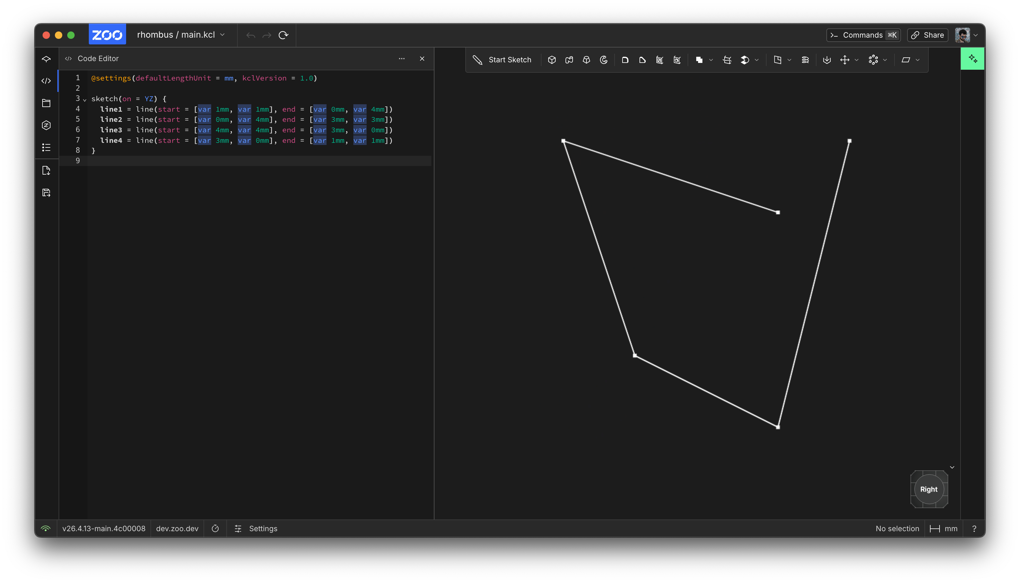
That doesn't look very much like a rhombus. Let's add some constraints -- some requirements we know. Firstly, we know that all 4 edges should share corners. In other words, line1 should end where line2 begins, line 2 should end where line 3 begins, and so on. Let's add some constraints with the coincident function.
@settings(defaultLengthUnit = mm, kclVersion = 1.0)

sketch(on = YZ) {
  line1 = line(start = [var 1mm, var 1mm], end = [var 0mm, var 4mm])
  line2 = line(start = [var 0mm, var 4mm], end = [var 3mm, var 3mm])
  line3 = line(start = [var 4mm, var 4mm], end = [var 3mm, var 0mm])
  line4 = line(start = [var 3mm, var 0mm], end = [var 1mm, var 1mm])

  // The 4 lines should form a shape, i.e. their endpoints should touch.
  coincident([line1.end, line2.start])
  coincident([line2.end, line3.start])
  coincident([line3.end, line4.start])
  coincident([line4.end, line1.start])
}
There, now our 4 lines form a quadrilateral.
What else do we know about a rhombus? Well, we know that opposite lines have to be parallel. So let's tell KCL that line1 and line3 are parallel, using KCL's parallel constraint. We add the parallel([line1, line3]) and parallel([line2, line4]) to our sketch block.
@settings(defaultLengthUnit = mm, kclVersion = 1.0)

sketch(on = YZ) {
  line1 = line(start = [var 1mm, var 1mm], end = [var 0mm, var 4mm])
  line2 = line(start = [var 0mm, var 4mm], end = [var 3mm, var 3mm])
  line3 = line(start = [var 4mm, var 4mm], end = [var 3mm, var 0mm])
  line4 = line(start = [var 3mm, var 0mm], end = [var 1mm, var 1mm])

  // The 4 lines should form a shape, i.e. their endpoints should touch.
  coincident([line1.end, line2.start])
  coincident([line2.end, line3.start])
  coincident([line3.end, line4.start])
  coincident([line4.end, line1.start])

  // Opposite edges are parallel.
  parallel([line1, line3])
  parallel([line2, line4])
}
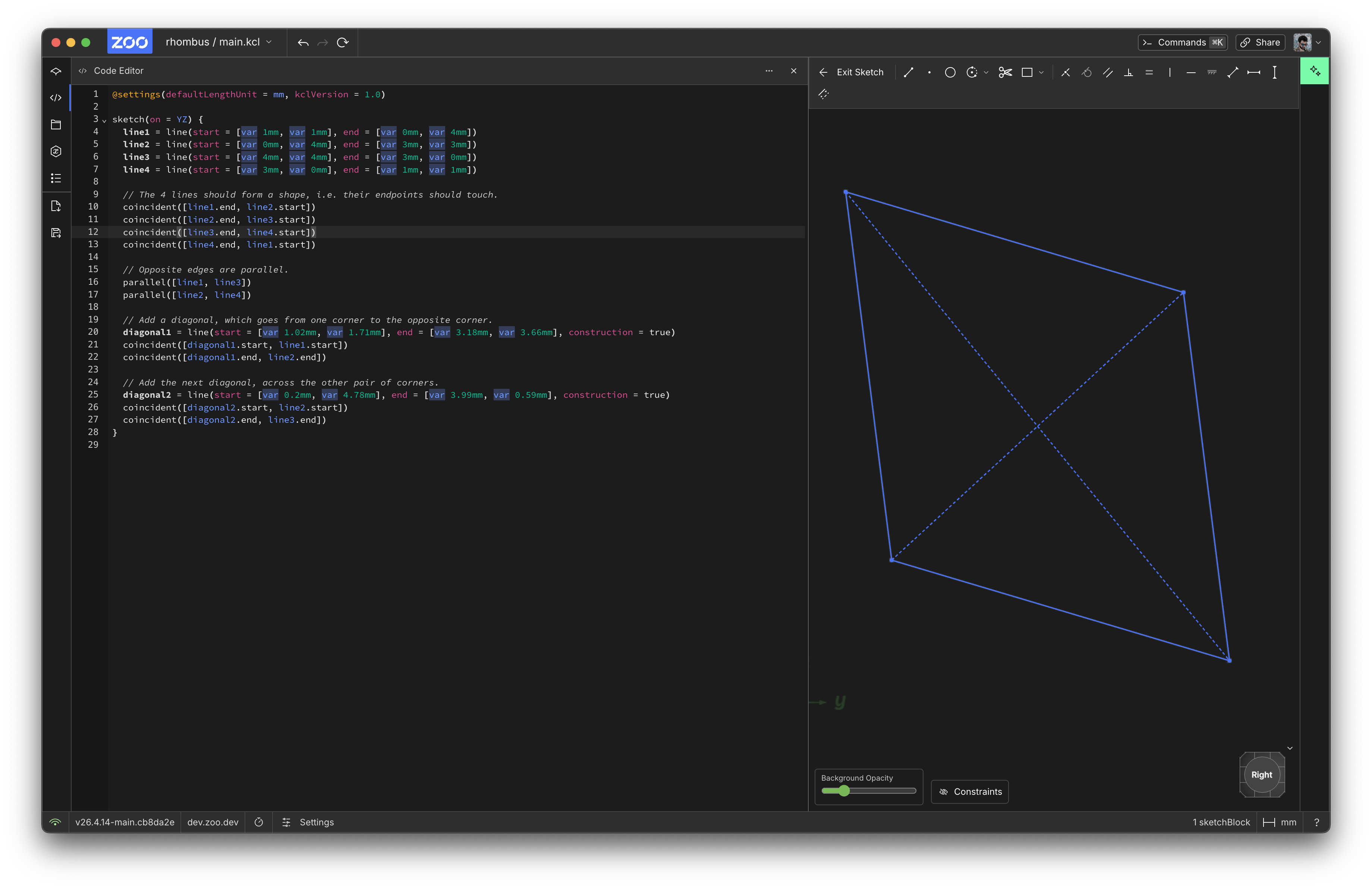
Lastly, their internal diagonals should be perpendicular. Firstly, let's define its diagonals:
// Add a diagonal, which goes from one corner to the opposite corner.
diagonal1 = line(
  start = [var 1.02mm, var 1.71mm],
  end = [var 3.18mm, var 3.66mm],
  // This line is construction geometry: not included in our final shape.
  // It's just used to constrain our real geometry.
  construction = true,
)
coincident([diagonal1.start, line1.start])
coincident([diagonal1.end, line2.end])

// Add the next diagonal, across the other pair of corners.
diagonal2 = line(
  start = [var 0.2mm, var 4.78mm],
  end = [var 3.99mm, var 0.59mm],
  // Again, this is construction geometry.
  construction = true,
)
coincident([diagonal2.start, line2.start])
coincident([diagonal2.end, line3.end])
We've marked these two diagonal lines as construction geometry. That means we don't want them to appear in the final rendered shape. We're only adding these lines to our sketch block for constraining other, real geometry. But it shouldn't actually make a selectable edge elsewhere in our design. If you view the sketch in Zoo Design Studio, construction geometry is drawn with dashed lines. Real geometry uses normal, full lines.
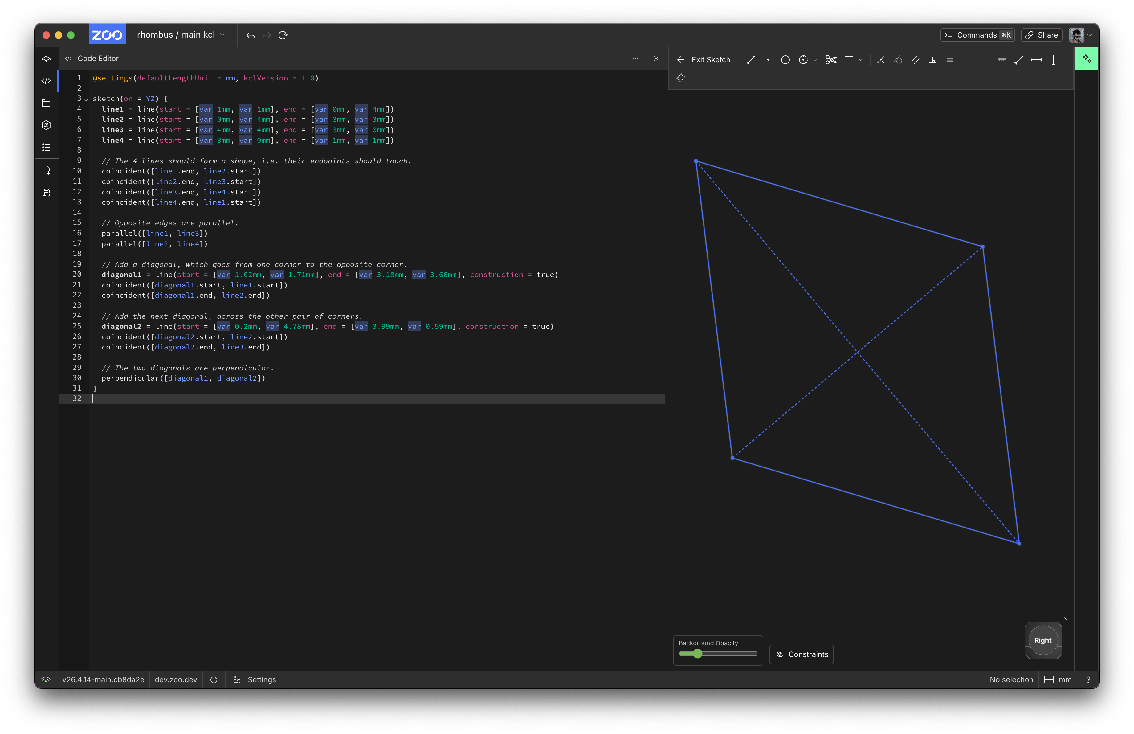
Let's add a perpendicular constraint on the diagonals:
// The two diagonals are perpendicular.
perpendicular([diagonal1, diagonal2])
Now our shape is properly constrained to be a rhombus! Here's the final result:
@settings(defaultLengthUnit = mm, kclVersion = 1.0)

starting = sketch(on = YZ) {
  line1 = line(start = [var 0.74mm, var 0.98mm], end = [var 0.13mm, var 3.79mm])
  line2 = line(start = [var 0.13mm, var 3.79mm], end = [var 2.98mm, var 3.33mm])
  line3 = line(start = [var 2.98mm, var 3.33mm], end = [var 3.58mm, var 0.51mm])
  line4 = line(start = [var 3.58mm, var 0.51mm], end = [var 0.74mm, var 0.98mm])

  // The 4 lines should form a shape, i.e. their endpoints should touch.
  coincident([line1.end, line2.start])
  coincident([line2.end, line3.start])
  coincident([line3.end, line4.start])
  coincident([line4.end, line1.start])

  // Opposite edges are parallel.
  parallel([line1, line3])
  parallel([line2, line4])

  // Add a diagonal, which goes from one corner to the opposite corner.
  diagonal1 = line(start = [var 0.74mm, var 0.98mm], end = [var 2.98mm, var 3.33mm], construction = true)
  coincident([diagonal1.start, line1.start])
  coincident([diagonal1.end, line2.end])

  // Add the next diagonal, across the other pair of corners.
  diagonal2 = line(start = [var 0.13mm, var 3.79mm], end = [var 3.58mm, var 0.51mm], construction = true)
  coincident([diagonal2.start, line2.start])
  coincident([diagonal2.end, line3.end])

  // The two diagonals are perpendicular.
  perpendicular([diagonal1, diagonal2])
}
Now when KCL runs this program, it'll take the initial guesses for each point (marked with var) and apply the constraints to figure out the final locations of all our geometry. This really helps simplify complicated 2D shapes.
Conclusion
We've learned how to use KCL to define 2D shapes:
- Sketches are on some plane, and KCL includes standard planes XY, YZ and XZ (and their negative versions, which point the third axis down instead of up).
- Start a sketch with a sketch block like
sketch(on = XY) { ... }. - Sketches call functions like
lineto make geometry. - Geometry can use fixed, exact points like
[2, 2], or they can vary the point's exact location later (like[var 2, var 2]). - You can assign geometry to variables, like
myLine = line(start = [2, 2], end = [3, 3]). - Constraints like
parallelreposition geometry, e.g.parallel([line1, line2]).
Next, we'll look at how to build curved lines, like arcs and circles. We'll use new constraints on them to make more realistic shapes.
Sketching curved lines
In the previous chapter, we sketched basic shapes, like a triangle and a rhombus. In this chapter, we'll look at some more interesting kinds of sketches you can do, using other KCL standard library functions.
Fixed arcs
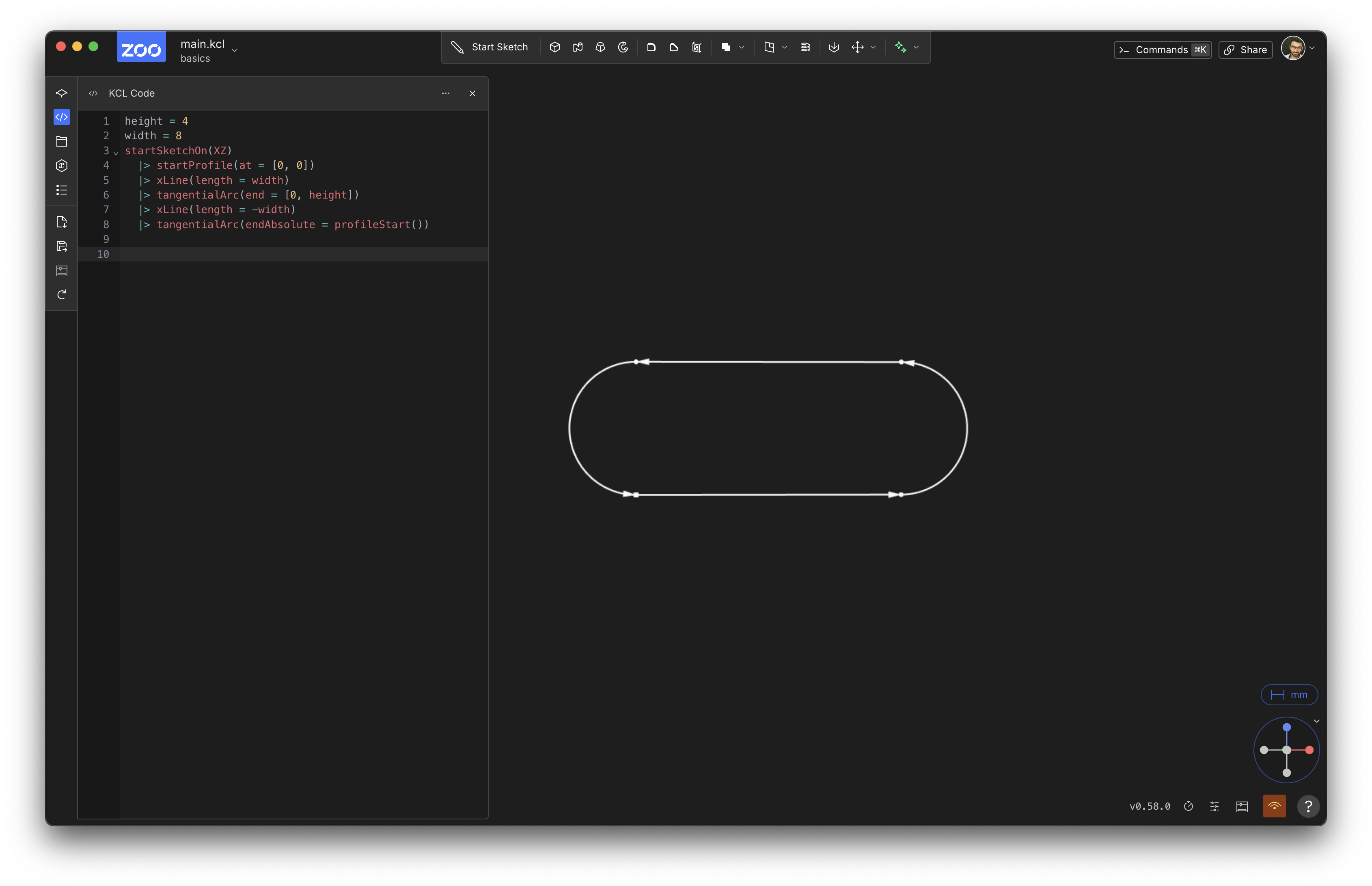
Let's sketch a pill shape, like a rectangle but with rounded edges. We'll need arcs for this! Let's start with a basic sketch with fixed size and position. We'll need two straight lines and two circular arcs, made with the arc function.
height = 4
width = 10
pill = sketch(on = XY) {
  bot = line(start = [0, 0], end = [width, 0])
  top = line(start = [0, height], end = [width, height])
  left = arc(start = [0, height], end = [0, 0], center = [0, height/2])
  right = arc(start = [width, 0], end = [width, height], center = [width, height/2])
}
In KCL, arcs are drawn counter-clockwise from their start point to their end point. This pill shape was very straightforward to code, but sketching it required me to use a pen and paper to figure out exactly where every point on the 2D plane was. The start and end of every arc and line had to be carefully calculated. Let's try letting KCL's constraint solver do the work for us instead.
Constrained arcs
We'll start again with two straight lines and two circular arcs, using some arbitrary values for each point's initial guess. I'm going to use Zoo Design Studio's UI to get these initial values, but you could guess them yourself, or do an approximate sketch on paper.
pill = sketch(on = YZ) {
  line1 = line(start = [var -4.15mm, var 5.79mm], end = [var 0.72mm, var 5.85mm])
  line2 = line(start = [var 0.92mm, var 4.16mm], end = [var -4.11mm, var 4.19mm])
  arc1 = arc(start = [var -4.9mm, var 5mm], end = [var -4.53mm, var 4.2mm], center = [var -3.93mm, var 4.97mm])
  arc2 = arc(start = [var 2.07mm, var 4.39mm], end = [var 1.96mm, var 5.77mm], center = [var 1.28mm, var 5.02mm])
}
Our first job is to connect these 4 segments together:
// Connect the 4 segments together
coincident([arc1.start, line1.start])
coincident([line1.end, arc2.end])
coincident([arc2.start, line2.start])
coincident([line2.end, arc1.end])
We know the pill should have parallel straight lines of equal length, so we'll add those constraints:
parallel([line1, line2])
equalLength([line1, line2])
We also want the two circular arcs to be the same radius, and to meet smoothly at the straight lines. So we'll add:
equalRadius([arc2, arc1])
tangent([line1, arc1])
tangent([line1, arc2])
Great! Our final shape should look like this:
pill = sketch(on = YZ) {
  line1 = line(start = [var -4.18mm, var 5.88mm], end = [var 1.34mm, var 5.85mm])
  line2 = line(start = [var 1.32mm, var 4.12mm], end = [var -4.19mm, var 4.15mm])
  arc1 = arc(start = [var -4.18mm, var 5.88mm], end = [var -4.19mm, var 4.15mm], center = [var -4.18mm, var 5.01mm])
  arc2 = arc(start = [var 1.32mm, var 4.12mm], end = [var 1.34mm, var 5.85mm], center = [var 1.33mm, var 4.99mm])
  coincident([arc1.start, line1.start])
  coincident([line1.end, arc2.end])
  coincident([arc2.start, line2.start])
  coincident([line2.end, arc1.end])
  parallel([line1, line2])
  equalLength([line1, line2])
  equalRadius([arc2, arc1])
  tangent([line1, arc1])
  tangent([line1, arc2])
}
This defines a nice pill shape. We could fix its position in 3D space by adding a coincident constraint between the start of a line, and the origin (referred to in KCL as a built-in constant, ORIGIN). Or we could constrain the distance from some point to the origin with the built-in distance, verticalDistance and horizontalDistance functions.
Circles
And lastly, let's look at the humble circle.
myCircleSketch = sketch(on = XZ) {
  circle1 = circle(start = [var 0mm, var 4mm], center = [var 0mm, var 0mm])
}

NOTE: This screenshot, like most screenshots that follow, is from an isometric perspective. It may look like an ellipse, but it's actually a circle. It would look like a circle from a heads-on angle.
The circle function takes center and start arguments. The start argument is just any point along the circle's circumference. It's helpful in the Zoo point-and-click sketching UI, because it lets you easily snap constraints like a distance to it. The circle's radius is defined implicitly by the distance from center to start point.
Modeling 3D shapes
Previous chapters covered designing 2D shapes. Now it's time to design 3D shapes!
3D shapes are usually made by adding depth to a 2D shape. There are two common ways engineers do this: by extruding or revolving 2D shapes into 3D. There's some less common ways too, including sweeps and lofts. In this chapter, we'll go through each of these! Let's get started with the most common method: extruding.
Regions and Extrudes
Extruding basically takes a 2D shape and pulls it up, stretching it upwards into the third dimension. Let's start with our existing 2D pill shape from the previous chapter:
height = 4
width = 10
pill = sketch(on = XY) {
  bot = line(start = [0, 0], end = [width, 0])
  top = line(start = [0, height], end = [width, height])
  left = arc(start = [0, height], end = [0, 0], center = [0, height/2])
  right = arc(start = [width, 0], end = [width, height], center = [width, height/2])
}
It should look like this:
Now we're going to extrude it up into the third axis, making a 3D solid.
pill = sketch(on = XZ) {
  line1 = line(start = [var -4.18mm, var 5.88mm], end = [var 1.34mm, var 5.85mm])
  line2 = line(start = [var 1.32mm, var 4.12mm], end = [var -4.19mm, var 4.15mm])
  arc1 = arc(start = [var -4.18mm, var 5.88mm], end = [var -4.19mm, var 4.15mm], center = [var -4.18mm, var 5.01mm])
  arc2 = arc(start = [var 1.32mm, var 4.12mm], end = [var 1.34mm, var 5.85mm], center = [var 1.33mm, var 4.99mm])
  coincident([arc1.start, line1.start])
  coincident([line1.end, arc2.end])
  coincident([arc2.start, line2.start])
  coincident([line2.end, arc1.end])
  parallel([line1, line2])
  equalLength([line1, line2])
  equalRadius([arc2, arc1])
  tangent([line1, arc1])
  tangent([line1, arc2])
}

// Add these lines!
region001 = region(point = pill.arc1.center, sketch = pill)
extrude001 = extrude(region001, length = 1)
You should see something like this:
NOTE: If you're reading this book online, the above graphic should be an interactive 3D model. You can use your mouse (or touchpad) to spin the model, zoom in and out, pan around the 3D scene, etc.
We added two different functions to our program: region and extrude. They work together: region lets you pick out a closed region of 2D space from your sketch, and extrude transforms that region into a 3D solid.
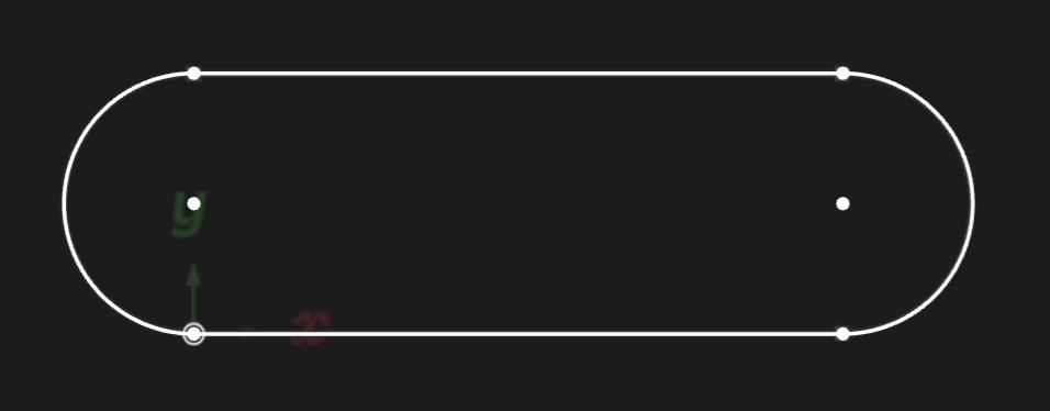
We need region because a sketch can contain lots of geometry. In the previous chapters, we used calls to line and arc to create closed shapes, like rhombuses and pills. But a sketch could contain multiple shapes, or free-floating lines that aren't part of any closed shape at all. Here's an example sketch:
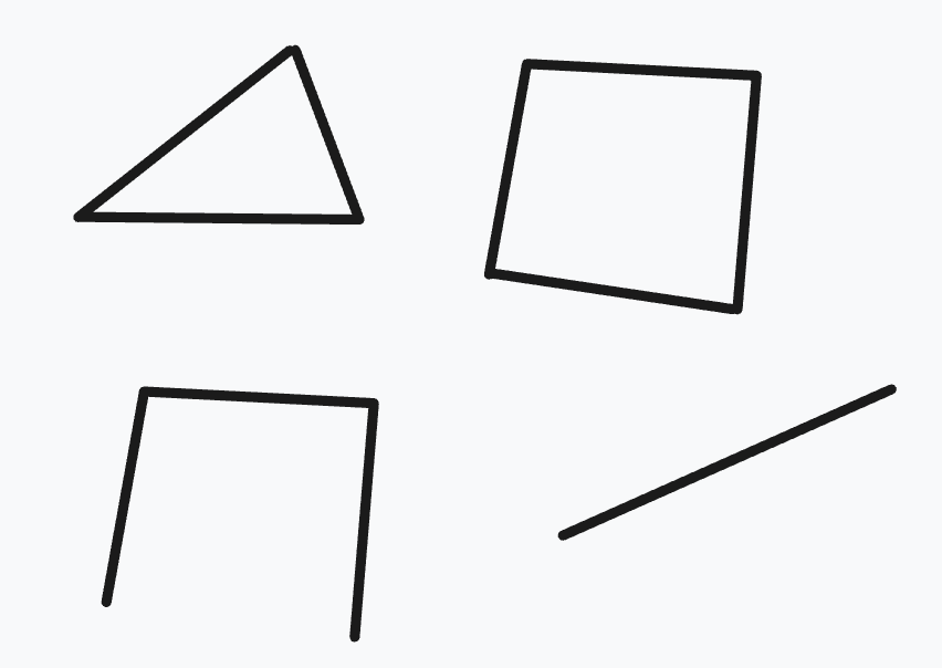
This sketch contains two closed shapes (a triangle and a square) as well as other lines. So, when we use the extrude function, we have to say which closed region we want to extrude. The region call takes in a point as its first parameter, and it returns the region that contains this point. If the point isn't actually in a closed region (in other words, if it's not surrounded by lines), the region call will return an error message.
You can pass either a named point, like point = pill.arc1.center, or a point literal (a 2D position, like point = [-1.44mm, 5.86mm]). We suggest you prefer named points over literal points, because if you edit your sketch, the exact boundaries of the geometry might change, and your target region might no longer enclose the specific position in your point literal!
NOTE: We're working on other ways to select regions, by choosing the lines (or arcs) that bound the region instead. We'll update this book when that API is ready.
Once you have a region of 2D space, you can turn that 2D space into 3D. We use the extrude function to take a region and say, "extrude it up into the 3rd dimension". extrude takes a distance, which is how far along the third axis to extrude. Every plane has a normal, or an axis which is tangent to the plane. For the plane XZ, this is the Y axis. This normal (also called the tangent, or the axis perpendicular to the plane), is the direction that extrude uses to add depth to your 2D region, making it 3D.
Advanced extrude options
bidirectionalLength = <number>: In addition to extruding up bylength, also extrude down by this much.symmetric = true: Instead of extruding up bylength, extrude up half the length, and down half the length. So, if you sketch onXYand thenextrude(length = 10), it'll extrude 10 fromZ=0toZ=10. But if you useextrude(length = 10, symmetric = true)it'll go fromZ=-5toZ=5.to = <target>: Set a target (you can use a point, axis, plane, edge, face, sketch or solid), and this will extrude until it makes the solid reach the target (or as close as it can possibly get).twistAngle = 30deg: While extruding, twist the sketch around its center. Or choose some other point to twist around, viatwistCenter. Change the twist speed withtwistAngleStep.
Sweep
An extrude takes some 2D region and drags it up in a straight line along the normal axis. A sweep is like an extrude, but the shape isn't just moved along a straight line: it could be moved along any path. Let's reuse our previous pill-shape example, but this time we'll sweep it instead of extruding it. First, we have to define a path that the sweep will take. Let's add one:
pillSketch = sketch(on = YZ) {
  line1 = line(start = [var -4.18mm, var 5.88mm], end = [var 1.34mm, var 5.85mm])
  line2 = line(start = [var 1.32mm, var 4.12mm], end = [var -4.19mm, var 4.15mm])
  arc1 = arc(start = [var -4.18mm, var 5.88mm], end = [var -4.19mm, var 4.15mm], center = [var -4.18mm, var 5.01mm])
  arc2 = arc(start = [var 1.32mm, var 4.12mm], end = [var 1.34mm, var 5.85mm], center = [var 1.33mm, var 4.99mm])
  coincident([arc1.start, line1.start])
  coincident([line1.end, arc2.end])
  coincident([arc2.start, line2.start])
  coincident([line2.end, arc1.end])
  parallel([line1, line2])
  equalLength([line1, line2])
  equalRadius([arc2, arc1])
  tangent([line1, arc1])
  tangent([line1, arc2])
}
pillRegion = region(point = [-1.44mm, 5.86mm], sketch = pillSketch)

pathSketch = sketch(on = XZ) {
  line1 = line(start = [var 0mm, var 5.06mm], end = [var -5.02mm, var 4.93mm])
  vertical([line1.start, ORIGIN])
  arc1 = arc(start = [var -4.54mm, var 12.82mm], end = [var -5.02mm, var 4.93mm], center = [var -5.12mm, var 8.9mm])
  coincident([line1.end, arc1.end])
  tangent([line1, arc1])
}

Our variable pathSketch has two lines (one straight line, one arc). Note that they don't form a region! They form an open profile, i.e. a sequence of lines that doesn't close back in on itself.
Now we'll add the sweep call, like sweep(pillRegion, path = [pathSketch.line1, pathSketch.arc1]), which will drag our 2D pill sketch along the path we defined. We'll add it to the bottom of our code:
// This is the same in the previous example program:
pillSketch = sketch(on = YZ) {
  line1 = line(start = [var -4.18mm, var 5.88mm], end = [var 1.34mm, var 5.85mm])
  line2 = line(start = [var 1.32mm, var 4.12mm], end = [var -4.19mm, var 4.15mm])
  arc1 = arc(start = [var -4.18mm, var 5.88mm], end = [var -4.19mm, var 4.15mm], center = [var -4.18mm, var 5.01mm])
  arc2 = arc(start = [var 1.32mm, var 4.12mm], end = [var 1.34mm, var 5.85mm], center = [var 1.33mm, var 4.99mm])
  coincident([arc1.start, line1.start])
  coincident([line1.end, arc2.end])
  coincident([arc2.start, line2.start])
  coincident([line2.end, arc1.end])
  parallel([line1, line2])
  equalLength([line1, line2])
  equalRadius([arc2, arc1])
  tangent([line1, arc1])
  tangent([line1, arc2])
}
pillRegion = region(point = [-1.44mm, 5.86mm], sketch = pillSketch)

pathSketch = sketch(on = XZ) {
  line1 = line(start = [var 0mm, var 5.06mm], end = [var -5.02mm, var 4.93mm])
  vertical([line1.start, ORIGIN])
  arc1 = arc(start = [var -4.54mm, var 12.82mm], end = [var -5.02mm, var 4.93mm], center = [var -5.12mm, var 8.9mm])
  coincident([line1.end, arc1.end])
  tangent([line1, arc1])
}

// Add this new line of code to your program!
// Sweep the pill-shaped region along the given path.
sweep(pillRegion, path = [pathSketch.line1, pathSketch.arc1])
Advanced sweep options
The sweep call has several other options you can set, listed in its documentation. Here are some optional parameters you can use to tweak the exact algorithm Zoo uses to compute the sweep:
relativeTo = sweep::TRAJECTORYorrelativeTo = sweep::SKETCH_PLANEaffects how the shape being swept will move along the path. This is optional and defaults tosweep::TRAJECTORY.version = 1orversion = 2will change which Zoo sweep algorithm to use. The default, 0, means the Zoo engine will use whichever it thinks is best. 1 is the version we first launched Zoo with, and 2 is a new improved version that works better in many cases.sectional = truewill divide the swept path into several different stages, one per line in the path. The default issectional = false.
If your sweep looks strange, try playing around with these options, or read the sweep docs page for more information.
Revolve
Revolves are another common way to make a 3D shape. Let's start with a 2D shape, like a basic circle.
circleSketch = sketch(on = XZ) {
  // Sketch a circle whose center is [20, 0].
  circle1 = circle(start = [var 0mm, var 1mm], center = [var 0mm, var 0mm])
  fixed([circle1.center, [20, 0]])

  // Use construction geometry to set the circle's radius to 1mm.
  vertical([circle1.start, circle1.center])
  line1 = line(start = [var 0mm, var 0mm], end = [var 0mm, var 1mm], construction = true)
  coincident([line1.start, circle1.center])
  coincident([line1.end, circle1.start])
  distance([line1.start, line1.end]) == 1mm
}

Note that we placed the circle at [20, 0], i.e. 20 units away from the global origin.
The revolve function takes a shape and revolves it, by dragging it around an axis. Let's revolve our circle around the Y axis (which is perpendicular to XZ, the plane we're sketching on), to make a ring shape. Because the circle being revolved is 20 units away from the global origin, the ring produced by the revolve should have a radius of 20.
circleSketch = sketch(on = XZ) {
  // Sketch a circle whose center is [20, 0].
  circle1 = circle(start = [var 0mm, var 1mm], center = [var 0mm, var 0mm])
  fixed([circle1.center, [20, 0]])

  // Use construction geometry to set the circle's radius to 1mm.
  vertical([circle1.start, circle1.center])
  line1 = line(start = [var 0mm, var 0mm], end = [var 0mm, var 1mm], construction = true)
  coincident([line1.start, circle1.center])
  coincident([line1.end, circle1.start])
  distance([line1.start, line1.end]) == 1mm
}

// Pick the region inside the circle
region001 = region(point = [20mm, -0.9975mm], sketch = circleSketch)

// Revolve it around the center of the scene
revolve001 = revolve(region001, axis = Y)
revolve has an optional argument called angle. In the above example, we didn't provide it, so it defaulted to 360 degrees. But we can set it to 240 degrees, and get two thirds of a donut:
// This part is the same as the previous example:
circleSketch = sketch(on = XZ) {
  circle1 = circle(start = [var 0mm, var 1mm], center = [var 0mm, var 0mm])
  fixed([circle1.center, [20, 0]])
  vertical([circle1.start, circle1.center])
  line1 = line(start = [var 0mm, var 0mm], end = [var 0mm, var 1mm], construction = true)
  coincident([line1.start, circle1.center])
  coincident([line1.end, circle1.start])
  distance([line1.start, line1.end]) == 1mm
}
region001 = region(point = [20mm, -0.9975mm], sketch = circleSketch)

// Change the angle to 240deg
revolve001 = revolve(region001, angle = 240deg, axis = Y)
Spheres
You can make a sphere by revolving a semicircle its full 360 degrees. First, let's make a semicircle:
semiCircleSketch = sketch(on = XZ) {
  arc1 = arc(start = [var 1.81mm, var -2.03mm], end = [var -1.91mm, var 1.94mm], center = [var 0mm, var 0mm])
  coincident([arc1.center, ORIGIN])
  line1 = line(start = [var 0mm, var 1.74mm], end = [var 0mm, var 0mm])
  vertical([line1.start, ORIGIN])
  coincident([line1.end, arc1.center])
  line2 = line(start = [var 0mm, var 0mm], end = [var 0mm, var -1.92mm])
  coincident([line2.start, line1.end])
  vertical([line2.end, ORIGIN])
  equalLength([line1, line2])
  distance([line1.start, line1.end]) == 1.83mm
  coincident([line1.start, arc1.end])
  coincident([arc1.start, line2.end])
}

Then we can revolve that semicircle 360 degrees to make a sphere:
semiCircleSketch = sketch(on = XZ) {
  arc1 = arc(start = [var 1.81mm, var -2.03mm], end = [var -1.91mm, var 1.94mm], center = [var 0mm, var 0mm])
  coincident([arc1.center, ORIGIN])
  line1 = line(start = [var 0mm, var 1.74mm], end = [var 0mm, var 0mm])
  vertical([line1.start, ORIGIN])
  coincident([line1.end, arc1.center])
  line2 = line(start = [var 0mm, var 0mm], end = [var 0mm, var -1.92mm])
  coincident([line2.start, line1.end])
  vertical([line2.end, ORIGIN])
  equalLength([line1, line2])
  distance([line1.start, line1.end]) == 1.83mm
  coincident([line1.start, arc1.end])
  coincident([arc1.start, line2.end])
}

semiCircleRegion = region(point = [1.8275mm, 0mm], sketch = semiCircleSketch)
revolve001 = revolve(semiCircleRegion, axis = Y)

Note that here, we omitted the angle argument from the revolve call because it defaults to 360 degrees.
Lofts
All previous methods -- extrudes, sweeps, revolves -- took a single 2D shape and made a single 3D solid. Lofts are a little different -- they take multiple 2D shapes and join them to make a single 3D shape. A loft interpolates between various sketches, creating a volume that smoothly blends from one shape into another. Let's see an example:
// Sketch a square
square = sketch(on = XY) {
  line1 = line(start = [var 0mm, var -2mm], end = [var 2mm, var -2mm])
  line2 = line(start = [var 2mm, var -2mm], end = [var 2mm, var 0mm])
  line3 = line(start = [var 2mm, var 0mm], end = [var 0mm, var 0mm])
  line4 = line(start = [var 0mm, var 0mm], end = [var 0mm, var -2mm])
  coincident([line1.end, line2.start])
  coincident([line2.end, line3.start])
  coincident([line3.end, line4.start])
  coincident([line4.end, line1.start])
  parallel([line2, line4])
  parallel([line3, line1])
  perpendicular([line1, line2])
  horizontal(line3)
  equalLength([line1, line2, line3, line4])
  perpendicular([line4, line1])
  coincident([line4.start, [-5mm, 5mm]])
  distance([line3.start, line3.end]) == 10mm
}

// Sketch a circle, 10mm above the square.
circle = sketch(on = offsetPlane(XY, offset = 10mm)) {
  circle1 = circle(start = [var 0mm, var 1.5mm], center = [var 0mm, var 0mm])
  coincident([circle1.center, ORIGIN])
  vertical([circle1.start, circle1.center])
  distance([circle1.start, circle1.center]) == 1.5mm
}

// Pick out the right regions from each sketch.
squareRegion = region(point = [0mm, -4.9975mm], sketch = square)
circleRegion = region(point = [0mm, -1.4975mm], sketch = circle)

// Loft the square into the circle.
loft([squareRegion, circleRegion])
offsetPlane function to start the circle sketch above the XY plane. We'll cover offsetPlane more in the chapter on planes. The loft function has a few other advanced options you can set. One of these is vDegree, which affects how smoothly KCL interpolates between the shapes. Take a look at these two examples, which are identical except for vDegree. This example uses vDegree = 1:
// Sketch a square
square = sketch(on = XY) {
  line1 = line(start = [var 0mm, var -2mm], end = [var 2mm, var -2mm])
  line2 = line(start = [var 2mm, var -2mm], end = [var 2mm, var 0mm])
  line3 = line(start = [var 2mm, var 0mm], end = [var 0mm, var 0mm])
  line4 = line(start = [var 0mm, var 0mm], end = [var 0mm, var -2mm])
  coincident([line1.end, line2.start])
  coincident([line2.end, line3.start])
  coincident([line3.end, line4.start])
  coincident([line4.end, line1.start])
  parallel([line2, line4])
  parallel([line3, line1])
  perpendicular([line1, line2])
  horizontal(line3)
  equalLength([line1, line2, line3, line4])
  perpendicular([line4, line1])
  coincident([line4.start, [-5mm, 5mm]])
  distance([line3.start, line3.end]) == 10mm
}

// Sketch a circle, 10mm above the square.
circle = sketch(on = offsetPlane(XY, offset = 10mm)) {
  circle1 = circle(start = [var 0mm, var 1.5mm], center = [var 0mm, var 0mm])
  coincident([circle1.center, ORIGIN])
  vertical([circle1.start, circle1.center])
  distance([circle1.start, circle1.center]) == 1.5mm
}

// Another square, above the other shapes.
square2 = sketch(on = offsetPlane(XY, offset = 20mm)) {
  line1 = line(start = [var 0mm, var -2mm], end = [var 2mm, var -2mm])
  line2 = line(start = [var 2mm, var -2mm], end = [var 2mm, var 0mm])
  line3 = line(start = [var 2mm, var 0mm], end = [var 0mm, var 0mm])
  line4 = line(start = [var 0mm, var 0mm], end = [var 0mm, var -2mm])
  coincident([line1.end, line2.start])
  coincident([line2.end, line3.start])
  coincident([line3.end, line4.start])
  coincident([line4.end, line1.start])
  parallel([line2, line4])
  parallel([line3, line1])
  perpendicular([line1, line2])
  horizontal(line3)
  equalLength([line1, line2, line3, line4])
  perpendicular([line4, line1])
  coincident([line4.start, [-5mm, 5mm]])
  distance([line3.start, line3.end]) == 10mm
}

// Pick out the right regions from each sketch.
squareRegion = region(point = [0mm, -4.9975mm], sketch = square)
circleRegion = region(point = [0mm, -1.4975mm], sketch = circle)
squareRegion2 = region(point = [0mm, -4.9975mm], sketch = square2)

// Loft the square into the circle.
loftedSolid = loft([squareRegion, circleRegion, squareRegion2], vDegree = 1)
vDegree = 2. That's actually the default, so we don't need to set it, but for the sake of example we'll explicitly set it there.
Click here for the same KCL code, but using vDegree = 2
// Sketch a square
square = sketch(on = XY) {
  line1 = line(start = [var 0mm, var -2mm], end = [var 2mm, var -2mm])
  line2 = line(start = [var 2mm, var -2mm], end = [var 2mm, var 0mm])
  line3 = line(start = [var 2mm, var 0mm], end = [var 0mm, var 0mm])
  line4 = line(start = [var 0mm, var 0mm], end = [var 0mm, var -2mm])
  coincident([line1.end, line2.start])
  coincident([line2.end, line3.start])
  coincident([line3.end, line4.start])
  coincident([line4.end, line1.start])
  parallel([line2, line4])
  parallel([line3, line1])
  perpendicular([line1, line2])
  horizontal(line3)
  equalLength([line1, line2, line3, line4])
  perpendicular([line4, line1])
  coincident([line4.start, [-5mm, 5mm]])
  distance([line3.start, line3.end]) == 10mm
}

// Sketch a circle, 10mm above the square.
circle = sketch(on = offsetPlane(XY, offset = 10mm)) {
  circle1 = circle(start = [var 0mm, var 1.5mm], center = [var 0mm, var 0mm])
  coincident([circle1.center, ORIGIN])
  vertical([circle1.start, circle1.center])
  distance([circle1.start, circle1.center]) == 1.5mm
}

// Another square, above the other shapes.
square2 = sketch(on = offsetPlane(XY, offset = 20mm)) {
  line1 = line(start = [var 0mm, var -2mm], end = [var 2mm, var -2mm])
  line2 = line(start = [var 2mm, var -2mm], end = [var 2mm, var 0mm])
  line3 = line(start = [var 2mm, var 0mm], end = [var 0mm, var 0mm])
  line4 = line(start = [var 0mm, var 0mm], end = [var 0mm, var -2mm])
  coincident([line1.end, line2.start])
  coincident([line2.end, line3.start])
  coincident([line3.end, line4.start])
  coincident([line4.end, line1.start])
  parallel([line2, line4])
  parallel([line3, line1])
  perpendicular([line1, line2])
  horizontal(line3)
  equalLength([line1, line2, line3, line4])
  perpendicular([line4, line1])
  coincident([line4.start, [-5mm, 5mm]])
  distance([line3.start, line3.end]) == 10mm
}

// Pick out the right regions from each sketch.
squareRegion = region(point = [0mm, -4.9975mm], sketch = square)
circleRegion = region(point = [0mm, -1.4975mm], sketch = circle)
squareRegion2 = region(point = [0mm, -4.9975mm], sketch = square2)

// Loft the square into the circle.
// This time use vDegree = 2. This is the default, so you don't actually
// need to set it. We're setting it here for the sake of example.
loftedSolid = loft([squareRegion, circleRegion, squareRegion2], vDegree = 2)
vDegree makes a big difference. You can view other options on the loft docs page.
Fillets, Chamfers and Edges
- Motivation: Applying a fillet
- Relationships between edges
- Edges between faces
- Chamfers
- Measuring geometry
Motivation: Applying a fillet
When you manufacture a part, you often want to smooth off its sharp edges, so they're rounded and won't accidentally cut someone who holds it. Let's say we're modeling a cube, like this:
// Sketch a square
width = 1
square = sketch(on = XY) {
  line1 = line(start = [width / 2, -width / 2], end = [width / 2, width / 2])
  line2 = line(start = [width / 2, width / 2], end = [-width / 2, width / 2])
  line3 = line(start = [-width / 2, width / 2], end = [-width / 2, -width / 2])
  line4 = line(start = [-width / 2, -width / 2], end = [width / 2, -width / 2])
}

// Extrude a cube.
regionCube = region(point = [0.4975mm, 0mm], sketch = square)
extrudeCube = extrude(regionCube, length = width)
It produces a cube like this:
line function calls, which were all assigned to variables (line1, line2, etc). When we extruded the square into a cube, the variables were copied into the solid, under .sketch.tags. So we can reference the edge created from line1 via .sketch.tags.line1, and apply a fillet to it.
// Sketch a square
width = 1
square = sketch(on = XY) {
  line1 = line(start = [width / 2, -width / 2], end = [width / 2, width / 2])
  line2 = line(start = [width / 2, width / 2], end = [-width / 2, width / 2])
  line3 = line(start = [-width / 2, width / 2], end = [-width / 2, -width / 2])
  line4 = line(start = [-width / 2, -width / 2], end = [width / 2, -width / 2])
}

// Extrude a cube.
regionCube = region(point = [0.4975mm, 0mm], sketch = square)
extrudeCube = extrude(regionCube, length = width)

// Fillet one edge
filletCube = fillet(extrudeCube, tags = extrudeCube.sketch.tags.line1, radius = 0.2)
The fillet function accepts an argument tags, which expects edges to fillet. You can pass in a single edge, like we did, or an array of edges like [extrudeCube.sketch.tags.line1, extrudeCube.sketch.tags.line2].
That program should produce a cube with one filleted edge, like this:
// Sketch a square
width = 1
square = sketch(on = XY) {
  line1 = line(start = [width / 2, -width / 2], end = [width / 2, width / 2])
  line2 = line(start = [width / 2, width / 2], end = [-width / 2, width / 2])
  line3 = line(start = [-width / 2, width / 2], end = [-width / 2, -width / 2])
  line4 = line(start = [-width / 2, -width / 2], end = [width / 2, -width / 2])
}

// Extrude a cube.
regionCube = region(point = [0.4975mm, 0mm], sketch = square)
extrudeCube = extrude(regionCube, length = width)

// Fillet all bottom edges
filletCube = fillet(
  extrudeCube,
  tags = [
    extrudeCube.sketch.tags.line1,
    extrudeCube.sketch.tags.line2,
    extrudeCube.sketch.tags.line3,
    extrudeCube.sketch.tags.line4,
  ],
  radius = 0.2,
)
Relationships between edges
So far, we've assigned geometry (like a line) to a variable when we create it, and then use that variable to refer to it later (e.g. for fillets). What about edges we don't create directly, and therefore can't assign to a variable? For example, we've already filleted the four bottom edges, but how do we fillet the top four edges? We aren't creating them via line calls. They're created by the CAD engine in the extrude call. If we didn't explicitly create them with a sketch function, how do we store them in a variable? Here's the secret --- you don't. KCL has a few helpful functions to access edges that you didn't create directly. Because we can refer to the bottom edges, we can use helper functions like getOppositeEdge to reference the top edges, like this:
// This is all the same as previous examples.
width = 1
square = sketch(on = XY) {
  line1 = line(start = [width / 2, -width / 2], end = [width / 2, width / 2])
  line2 = line(start = [width / 2, width / 2], end = [-width / 2, width / 2])
  line3 = line(start = [-width / 2, width / 2], end = [-width / 2, -width / 2])
  line4 = line(start = [-width / 2, -width / 2], end = [width / 2, -width / 2])
}
regionCube = region(point = [0.4975mm, 0mm], sketch = square)
extrudeCube = extrude(regionCube, length = width)

// Note that here we're using `getOppositeEdge`.
filletCube = fillet(
  extrudeCube,
  tags = [
    // Fillet the bottom edge
    extrudeCube.sketch.tags.line1,
    // Fillet the top edge
    getOppositeEdge(extrudeCube.sketch.tags.line1)
  ],
  radius = 0.2,
)
getOppositeEdge on each:
// Same as previous examples:
width = 1
square = sketch(on = XY) {
  line1 = line(start = [width / 2, -width / 2], end = [width / 2, width / 2])
  line2 = line(start = [width / 2, width / 2], end = [-width / 2, width / 2])
  line3 = line(start = [-width / 2, width / 2], end = [-width / 2, -width / 2])
  line4 = line(start = [-width / 2, -width / 2], end = [width / 2, -width / 2])
}
regionCube = region(point = [0.4975mm, 0mm], sketch = square)
extrudeCube = extrude(regionCube, length = width)

// Fillet edges
filletCube = fillet(
  extrudeCube,
  tags = [
    // Fillet the bottom four edges
    extrudeCube.sketch.tags.line1,
    extrudeCube.sketch.tags.line2,
    extrudeCube.sketch.tags.line3,
    extrudeCube.sketch.tags.line4,
    // Fillet the top four edges
    getOppositeEdge(extrudeCube.sketch.tags.line1),
    getOppositeEdge(extrudeCube.sketch.tags.line2),
    getOppositeEdge(extrudeCube.sketch.tags.line3),
    getOppositeEdge(extrudeCube.sketch.tags.line4)
  ],
  radius = 0.2,
)
getNextAdjacentEdge and getPreviousAdjacentEdge to reference them:
// Sketch a square
width = 1
square = sketch(on = XY) {
  line1 = line(start = [width / 2, -width / 2], end = [width / 2, width / 2])
  line2 = line(start = [width / 2, width / 2], end = [-width / 2, width / 2])
  line3 = line(start = [-width / 2, width / 2], end = [-width / 2, -width / 2])
  line4 = line(start = [-width / 2, -width / 2], end = [width / 2, -width / 2])
}

// Extrude a cube
regionCube = region(point = [0.4975mm, 0mm], sketch = square)
extrudeCube = extrude(regionCube, length = width)

// Fillet edges
filletCube = fillet(
  extrudeCube,
  tags = [
    // Bottom edge
    extrudeCube.sketch.tags.line1,
    // One side edge
    getNextAdjacentEdge(extrudeCube.sketch.tags.line1),
    // The other side edge
    getPreviousAdjacentEdge(extrudeCube.sketch.tags.line1),
  ],
  radius = 0.2,
)
line1 just like we did before. But we've also filleted the sides adjacent to it. One side is "before" line1, one side is "after" line1, in Zoo's internal tracking of edges. We can use a similar trick to fillet all four vertical side edges:
// Sketch a square
width = 1
square = sketch(on = XY) {
  line1 = line(start = [width / 2, -width / 2], end = [width / 2, width / 2])
  line2 = line(start = [width / 2, width / 2], end = [-width / 2, width / 2])
  line3 = line(start = [-width / 2, width / 2], end = [-width / 2, -width / 2])
  line4 = line(start = [-width / 2, -width / 2], end = [width / 2, -width / 2])
}

// Extrude a cube
regionCube = region(point = [0.4975mm, 0mm], sketch = square)
extrudeCube = extrude(regionCube, length = width)

// Fillet edges
filletCube = fillet(
  extrudeCube,
  tags = [
    getNextAdjacentEdge(extrudeCube.sketch.tags.line1),
    getPreviousAdjacentEdge(extrudeCube.sketch.tags.line1),
    getNextAdjacentEdge(extrudeCube.sketch.tags.line2),
    getPreviousAdjacentEdge(extrudeCube.sketch.tags.line3),
  ],
  radius = 0.2,
)
Edges between faces
Sometimes getNextAdjacentEdge and similar functions are a bit tricky to use. It can be hard to look at a model and figure out which is the next, or previous, or opposite, edge. There's another way to refer to edges: which faces does this edge touch? For this we use the getCommonEdge function.
// This is the same as previous examples
width = 1
square = sketch(on = XY) {
  line1 = line(start = [width / 2, -width / 2], end = [width / 2, width / 2])
  line2 = line(start = [width / 2, width / 2], end = [-width / 2, width / 2])
  line3 = line(start = [-width / 2, width / 2], end = [-width / 2, -width / 2])
  line4 = line(start = [-width / 2, -width / 2], end = [width / 2, -width / 2])
}
regionCube = region(point = [0.4975mm, 0mm], sketch = square)
extrudeCube = extrude(regionCube, length = width)

// Find the edge that borders the face from line1 and the face from line2.
edge = getCommonEdge(faces = [
  extrudeCube.sketch.tags.line1,
  extrudeCube.sketch.tags.line2
])

// Then fillet it.
fillet(extrudeCube, tags = edge, radius = 0.2)
getCommonEdge takes a list of faces, and returns the edge that is shared between them -- their common edge. This is a pretty useful function, because usually it's easier to reference and name faces rather than edges.
Notice in this example that the list of faces looks like a list of edges. We're passing in line1 and line2, which we used to reference edges in the above examples. That's because KCL recognizes that extrude creates a face out of each edge (imagine each edge being dragged upwards, to create a face).
There are other ways to refer to faces, but we'll see them later in this book.
Chamfers
A chamfer is just like a fillet, except that fillets smooth away an edge to make it round, but chamfers just make a single cut across an edge. Here's an example of the difference. Compare this chamfered cube with the filleted cubes above:
// Same as previous examples
width = 1
square = sketch(on = XY) {
  line1 = line(start = [width / 2, -width / 2], end = [width / 2, width / 2])
  line2 = line(start = [width / 2, width / 2], end = [-width / 2, width / 2])
  line3 = line(start = [-width / 2, width / 2], end = [-width / 2, -width / 2])
  line4 = line(start = [-width / 2, -width / 2], end = [width / 2, -width / 2])
}
regionCube = region(point = [0.4975mm, 0mm], sketch = square)
extrudeCube = extrude(regionCube, length = width)

// Apply a chamfer
chamferedCube = chamfer(extrudeCube, tags = [getOppositeEdge(extrudeCube.sketch.tags.line1)], length = 0.2)
Advanced chamfers
To define the chamfer, you only need to provide its length. But if you want more control of the chamfer angle, you can set the optional secondLength or angle parameters. Let's see how they work.
Chamfering cuts away at two faces, creating a third face in between them. By default, the chamfer cuts away an even amount from both sides, creating a chamfered face at a 45 degree angle. The amount cut away from each face is the length parameter. But you can make a chamfer that cuts different amounts from each face, using the secondLength or angle parameters. This diagram shows the cross-section of a cube being chamfered:
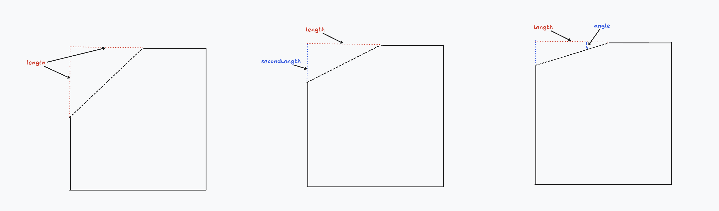
Setting a second length which is much bigger or smaller than the first length means the chamfer will be "steep" -- the new face will be at a very sharp (or very obtuse) angle between the existing two faces. You can also set this angle explicitly, via the angle parameter. You can't use both angle and secondLength because they're essentially two different ways of setting the same property.
Measuring geometry
So we've learned to use variables from sketch blocks to reference the lines we create, then use helper functions like getOppositeEdge to reference other geometry elsewhere in the model. But these variables aren't just used for altering edges. They provide a valuable way to query and measure your models. Let's see how.
Let's say you've got a solid triangle, like this:
// Make a triangle
sketch001 = sketch(on = YZ) {
  line1 = line(start = [var 5.29mm, var -4.11mm], end = [var -4.31mm, var -4.11mm])
  line2 = line(start = [var -4.31mm, var -4.11mm], end = [var 0.49mm, var 5.14mm])
  coincident([line1.end, line2.start])
  line3 = line(start = [var 0.49mm, var 5.14mm], end = [var 5.29mm, var -4.11mm])
  coincident([line2.end, line3.start])
  coincident([line3.end, line1.start])
  equalLength([line2, line3])
  horizontal(line1)
}

// Extrude it
region001 = region(point = [0.49mm, -4.1075mm], sketch = sketch001)
extrude001 = extrude(region001, length = 1)
Let's ask a simple question. How long is each side of the triangle?
It sounds simple, but to actually calculate it, you'd have to break out a pencil and paper, then do some trigonometry. The problem is, the length doesn't appear anywhere in the line function call. The lines are defined by their start and end points, and the length is an implicit property of those. Defining lines as a start and end is helpful, but it means important properties, like length, can't be read from our source code.
However, tags give us a simple way to refer to each line, and then query them for properties like length with the segLen function. Let's update our program:
// Make a triangle
sketch001 = sketch(on = YZ) {
  line1 = line(start = [var 5.29mm, var -4.11mm], end = [var -4.31mm, var -4.11mm])
  line2 = line(start = [var -4.31mm, var -4.11mm], end = [var 0.49mm, var 5.14mm])
  coincident([line1.end, line2.start])
  line3 = line(start = [var 0.49mm, var 5.14mm], end = [var 5.29mm, var -4.11mm])
  coincident([line2.end, line3.start])
  coincident([line3.end, line1.start])
  equalLength([line2, line3])
  horizontal(line1)
}
// Extrude it
region001 = region(point = [0.49mm, -4.1075mm], sketch = sketch001)
extrude001 = extrude(region001, length = 1)

// Measure its side lengths
side1Len = segLen(extrude001.sketch.tags.line1)
side2Len = segLen(extrude001.sketch.tags.line2)
side3Len = segLen(extrude001.sketch.tags.line3)
Now you can open up the Variables pane and look at the side1Len, side2Len and side3Len variables to find each side's length. That's pretty useful! And if you want to use those lengths elsewhere in your code, you can! You could start drawing lines where the end is [side1Len, 0] for example, or plug those lengths into other calculations.
There are other helpers too, like segStart and segEnd to find a line's start and end, respectively. Take a look at the KCL standard library docs to find them all.
Sketch on face
In the previous chapter, we looked at how leveraging KCL tags lets you query your edges (to find their length, or angle with the previous edge), or apply an edge cut (like a fillet or chamfer). But you can also tag more than just edges! In this chapter, we'll learn how to tag faces, and how that lets you build more complicated 3D models.
Side faces
Let's start with a simple example. First, we'll sketch and extrude a triangle.
// Make a triangle
sketch001 = sketch(on = YZ) {
  line1 = line(start = [var 5.29mm, var -4.11mm], end = [var -4.31mm, var -4.11mm])
  line2 = line(start = [var -4.31mm, var -4.11mm], end = [var 0.49mm, var 5.14mm])
  coincident([line1.end, line2.start])
  line3 = line(start = [var 0.49mm, var 5.14mm], end = [var 5.29mm, var -4.11mm])
  coincident([line2.end, line3.start])
  coincident([line3.end, line1.start])
  equalLength([line2, line3])
  horizontal(line1)
}

// Extrude it
region001 = region(point = [0.49mm, -4.1075mm], sketch = sketch001)
extrude001 = extrude(region001, length = 1)
line1 can be referred to via extrude001.sketch.tags.line1. We can use this to reference this face in our 3D model.
Now, if we want to start a new sketch on that face, we can do so, with the faceOf function!
myFace = faceOf(extrude001, face = region001.tags.line3)
sketch003 = sketch(on = myFace) {
  // We'll add lines to this sketch later.
}
In all the previous example sketches, we've sketched on a plane (like XY or YZ). But now, we're passing a solid face (of our extruded triangle) instead. The solid has five faces (three side faces, a bottom, and a top), so we use faceOf to say which face in particular we want to sketch on. As we discussed above, the face can be referenced via line1 (the line that it was extruded from). Now we can start sketching on this face, and even extrude that sketch too.
// Make a triangle
sketch001 = sketch(on = YZ) {
  line1 = line(start = [var 5.29mm, var -4.11mm], end = [var -4.31mm, var -4.11mm])
  line2 = line(start = [var -4.31mm, var -4.11mm], end = [var 0.49mm, var 5.14mm])
  coincident([line1.end, line2.start])
  line3 = line(start = [var 0.49mm, var 5.14mm], end = [var 5.29mm, var -4.11mm])
  coincident([line2.end, line3.start])
  coincident([line3.end, line1.start])
  equalLength([line2, line3])
  horizontal(line1)
}

// Extrude it
region001 = region(point = [0.49mm, -4.1075mm], sketch = sketch001)
extrude001 = extrude(region001, length = 1)

// Sketch on a face of the triangle.
face002 = faceOf(extrude001, face = region001.tags.line3)
sketch003 = sketch(on = face002) {
  line1 = line(start = [var -3.21mm, var 0mm], end = [var -2.7mm, var 0.65mm])
  horizontal([line1.start, ORIGIN])
  line2 = line(start = [var -2.7mm, var 0.65mm], end = [var -2.45mm, var 0.35mm])
  coincident([line1.end, line2.start])
  line3 = line(start = [var -2.45mm, var 0.35mm], end = [var -3.21mm, var 0mm])
  coincident([line2.end, line3.start])
  coincident([line3.end, line1.start])
}

// Extrude that sketch
region002 = region(point = [-2.9530332mm, 0.3234568mm], sketch = sketch003)
extrude002 = extrude(region002, length = 2)
Note: When you sketch on a face, the sketch uses the global coordinate system. This means when you use 2D points in your sketches, they're relative to the overall global scene, and not the face you're sketching on.
Sketching on faces is a really common pattern when designing real-world objects. A LEGO brick is a good example -- first you'd sketch the rectangular brick, then you'd sketch on its top face, adding the little bumps on top. But wait a second. How would we specify the top face of the brick? That face isn't created from any particular edge. So we can't tag its line call and then reuse that tag for the face. What should we do?
Standard faces
There's a simple solution to sketching on the top face. KCL has some built-in identifiers for the top and bottom face, END and START. We prefer the terms "start" and "end" to "top" and "bottom" because the latter depend on your camera angle, so they can be ambiguous. "Start" always refers to the original face from your 2D sketch. "End" always refers to the new face created at the end of the extrusion. Let's use them!
// Same as previous example
sketch001 = sketch(on = YZ) {
  line1 = line(start = [var 5.29mm, var -4.11mm], end = [var -4.31mm, var -4.11mm])
  line2 = line(start = [var -4.31mm, var -4.11mm], end = [var 0.49mm, var 5.14mm])
  coincident([line1.end, line2.start])
  line3 = line(start = [var 0.49mm, var 5.14mm], end = [var 5.29mm, var -4.11mm])
  coincident([line2.end, line3.start])
  coincident([line3.end, line1.start])
  equalLength([line2, line3])
  horizontal(line1)
}
region001 = region(point = [0.49mm, -4.1075mm], sketch = sketch001)
extrude001 = extrude(region001, length = 1)

// Changed: We're using `face = END` here, which is a built-in
// identifier for the end of an extrusion.
face002 = faceOf(extrude001, face = END)
sketch003 = sketch(on = face002) {
  line1 = line(start = [var -0.3mm, var 0.76mm], end = [var -1.26mm, var -1.25mm])
  line2 = line(start = [var -1.26mm, var -1.25mm], end = [var 1.68mm, var -1.14mm])
  coincident([line1.end, line2.start])
  line3 = line(start = [var 1.68mm, var -1.14mm], end = [var -0.3mm, var 0.76mm])
  coincident([line2.end, line3.start])
  coincident([line3.end, line1.start])
}

// Extrude that sketch
region002 = region(point = [-0.7777441mm, -0.2460774mm], sketch = sketch003)
extrude002 = extrude(region002, length = 1)
Tags
When you chamfer an edge, it creates a new face, which can also be sketched on! But before we do, we've got to take a quick detour and talk about tags.
When Zoo launched, tags were used a lot. These days, you probably won't ever need to use tags very much, if at all, because they've been mostly replaced by variables. There are still a few cases where you'll need tags, and sketching on a chamfered face is one of them. We're trying to phase them out, but we haven't finished that job yet.
So far, we've been able to refer to geometric features (like edges and faces) by using variables. But tags let you refer to geometry that isn't assigned to a variable. For example, take the chamfered face created by a chamfer(myRegion) call. When we call mySolid = chamfer(myRegion, length = 1) the variable mySolid refers to the entire solid, including the chamfered face. How do we refer to some specific face, like the chamfered face?
The solution: we use mySolid = chamfer(myRegion, length = 1, tag = $myFace). That tags the face, so we can refer to it later as myFace. You can think of this like declaring a variable inside the function, when it executes. The $ means you're declaring a tag. So, $myFace declares a tag called myFace. If you later use just myFace, you're referring to a tag that already exists.
Here's another example. Say you extrude a square into a cube. As discussed above, the top of the cube can be referred to with the standard face END. You can sketch on that top face via sketch(on = faceOf(extrude001, face = END)). Say you extrude a cylinder from the cube. How do you sketch on the top face of the cylinder? Does END refer to the cylinder, or the cube?
You can use extrude(mySketch, tagEnd = $endOfCylinder) to disambiguate these. Again, this defines a tag as part of the extrude, which refers to a particular face. Then you can use that tag later when you need to use the face.
Generally you won't need to use this method, but there are some niches where it's helpful.
Sketch on chamfer
Now that we understand tags, we can use them to sketch on a chamfer! When you chamfer an edge, it creates a new face, which can also be sketched on! Consider this chamfered cube from the previous chapter:
// Same as previous examples
width = 1
square = sketch(on = XY) {
  line1 = line(start = [width / 2, -width / 2], end = [width / 2, width / 2])
  line2 = line(start = [width / 2, width / 2], end = [-width / 2, width / 2])
  line3 = line(start = [-width / 2, width / 2], end = [-width / 2, -width / 2])
  line4 = line(start = [-width / 2, -width / 2], end = [width / 2, -width / 2])
}
regionCube = region(point = [0.4975mm, 0mm], sketch = square)
extrudeCube = extrude(regionCube, length = width)

// Apply a chamfer
chamferedCube = chamfer(
  extrudeCube,
  tags = [getOppositeEdge(extrudeCube.sketch.tags.line1)],
  length = 0.2,
)
chamfer call. Then we can use it in faceOf, and then we can sketch on it like any other face.
// Same as previous examples
width = 1
square = sketch(on = XY) {
  line1 = line(start = [width / 2, -width / 2], end = [width / 2, width / 2])
  line2 = line(start = [width / 2, width / 2], end = [-width / 2, width / 2])
  line3 = line(start = [-width / 2, width / 2], end = [-width / 2, -width / 2])
  line4 = line(start = [-width / 2, -width / 2], end = [width / 2, -width / 2])
}
regionCube = region(point = [0.4975mm, 0mm], sketch = square)
extrudeCube = extrude(regionCube, length = width)

// Apply a chamfer
chamferedCube = chamfer(
  extrudeCube,
  tags = [getOppositeEdge(extrudeCube.sketch.tags.line1)],
  length = 0.2,
  // Add a tag to the chamfered face:
  tag = $myChamferedFace,
)

// Refer back to the tagged face
faceToSketchOn = faceOf(extrudeCube, face = myChamferedFace)

// Start sketching on that face.
triangle = sketch(on = faceToSketchOn) {
  line1 = line(start = [var -0.37mm, var 0.33mm], end = [var -0.2mm, var 0.47mm])
  line2 = line(start = [var -0.2mm, var 0.47mm], end = [var 0.26mm, var 0.29mm])
  coincident([line1.end, line2.start])
  line3 = line(start = [var 0.26mm, var 0.29mm], end = [var -0.37mm, var 0.33mm])
  coincident([line2.end, line3.start])
  coincident([line3.end, line1.start])
}
region001 = region(point = [-0.2834107mm, 0.3980702mm], sketch = triangle)
extrude001 = extrude(region001, length = 0.4)
Updating bodies, or creating new bodies?
When you extrude a sketch from a face, you could be trying to do one of two things:
- Mutating the original body, by adding a new extrusion to it
- Creating a totally new body, which just happens to be touching the previous body.
Here's an example. Say you extrude a square into a cube, and then you extrude a cylinder out of the cube. Should the cylinder be its own separate body? Or should there be a single body, with a cube volume and a cylindrical volume? Here's a visual:
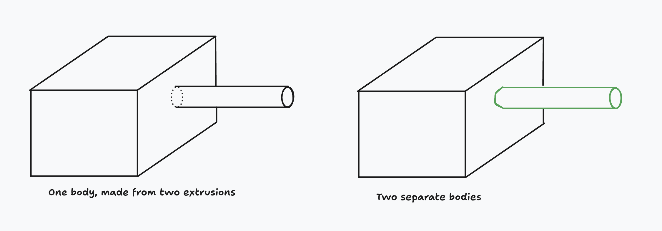
By default, extruding a sketch which was sketched on a face will merge the extrusion into the original body. In other words, the example on the left. But you can choose to make a new body instead (the example on the right). You can choose between this by setting the extrude method.
- Use
extrude(method = MERGE)(the default) to update the original solid. - Use
extrude(method = NEW)(an optional override) to create a new solid instead.
What's the practical difference between these? If you use MERGE, you've got one body. That means the single unified body will be translated, or rotated, or have its color changed, as one cohesive whole. With NEW, you've got two bodies, so you can reposition them independently, color them differently, etc. You'll learn how to move, rotate and recolor solids in the chapter on transforms.
OK! Now we've learned how to sketch on all sorts of things:
- Standard planes like XY or -XZ
- Tagged faces of existing solids
- Top or bottom faces of solids, using
STARTandEND - Chamfered faces cut out of solids, by tagging the
chamfercall
There's one more thing we can sketch on: custom planes. Let's learn more about planes in the next chapter.
Planes
A plane is a 2D surface that exists in 3D space. KCL has its own plane type, which is mostly used for starting a sketch. We've previously sketched on standard planes like XY (remember, there are six -- XY, YZ, XZ, -XY, -YZ and -XZ). But you can easily define your own planes too! We'll look at custom planes in this chapter.
Offset planes
You can use the offsetPlane function to copy any other plane, but moved some direction up or down the third axis. For example, let's draw a small circle on XY, a medium circle on a plane 10 units above it, and a big circle 20 units above it.
r = 10
sketch001 = sketch(on = XY) {
  circle1 = circle(start = [var -0.52mm, var 0.56mm], center = [var 0mm, var 0mm])
  coincident([circle1.center, ORIGIN])
  // Construction geometry line, used for the radius constraint.
  radiusLine = line(start = [var -0.52mm, var 0.56mm], end = [var 0mm, var 0mm], construction = true)
  coincident([radiusLine.start, circle1.start])
  coincident([radiusLine.end, circle1.center])
  // Constrain the circle's radius.
  distance([radiusLine.start, radiusLine.end]) == r
  vertical(radiusLine)
}

// Note the `offsetPlane` call!
sketch002 = sketch(on = offsetPlane(XY, offset = 10)) {
  circle1 = circle(start = [var -0.52mm, var 0.56mm], center = [var 0mm, var 0mm])
  coincident([circle1.center, ORIGIN])
  line1 = line(start = [var -0.52mm, var 0.56mm], end = [var 0mm, var 0mm], construction = true)
  coincident([line1.start, circle1.start])
  coincident([line1.end, circle1.center])
  distance([line1.start, line1.end]) == r * 2
  vertical(line1)
}

// Another `offsetPlane` call, offset even further!
sketch003 = sketch(on = offsetPlane(XY, offset = 20)) {
  circle1 = circle(start = [var -0.52mm, var 0.56mm], center = [var 0mm, var 0mm])
  coincident([circle1.center, ORIGIN])
  line1 = line(start = [var -0.52mm, var 0.56mm], end = [var 0mm, var 0mm], construction = true)
  coincident([line1.start, circle1.start])
  coincident([line1.end, circle1.center])
  distance([line1.start, line1.end]) == r * 3
  vertical(line1)
}
Custom planes
You can define your own plane with your own axes like this:
customPlane = {
  origin = { x = 0, y = 1, z = 0},
  xAxis = { x = 1, y = 0, z = 0 },
  yAxis = { x = 0, y = 0, z = 1 },
}
Note the custom plane has a few properties:
- An origin, which is a 3D point in space, using the global coordinate system (i.e. it's relative to the overall scene)
- X and Y axes, which are defined as vectors
The plane's Z axis is the cross product of its X and Y axes. It's uniquely determined, so you don't need to specify it. The Z axis respects the right-hand rule.
Now let's use this custom plane in a sketch. We'll build two identical cylinders, but one is on the standard XY plane, and one is on the custom plane we defined above.
customPlane = {
  origin = { x = 0, y = 6, z = 0 },
  xAxis = { x = 1, y = 0.5, z = 0 },
  yAxis = { x = 0, y = 0.5, z = 1 }
}

// Build a cylinder on a custom plane
sketch001 = sketch(on = customPlane) {
  circle1 = circle(start = [var -0.52mm, var 0.56mm], center = [var 0mm, var 0mm])
  coincident([circle1.center, ORIGIN])
  line1 = line(start = [var -0.52mm, var 0.56mm], end = [var 0mm, var 0mm], construction = true)
  coincident([line1.start, circle1.start])
  coincident([line1.end, circle1.center])
  distance([line1.start, line1.end]) == 1
  vertical(line1)
}
region001 = region(point = [0mm, -0.9975mm], sketch = sketch001)
extrude001 = extrude(region001, length = 2)

// Build the same cylinder, but on the XY plane.
sketch002 = sketch(on = XY) {
  circle1 = circle(start = [var -0.52mm, var 0.56mm], center = [var 0mm, var 0mm])
  coincident([circle1.center, ORIGIN])
  line1 = line(start = [var -0.52mm, var 0.56mm], end = [var 0mm, var 0mm], construction = true)
  coincident([line1.start, circle1.start])
  coincident([line1.end, circle1.center])
  distance([line1.start, line1.end]) == 1
  vertical(line1)
}
region002 = region(point = [0mm, -0.9975mm], sketch = sketch002)
extrude002 = extrude(region002, length = 2)
offsetPlane if you've already defined a plane on the same X and Y axis. You can even combine offsetPlane and custom planes, like this:
// Make a custom plane.
customPlane = {
  origin = { x = 0, y = 1, z = 0},
  xAxis = { x = 1, y = 0, z = 0 },
  yAxis = { x = 0, y = 0, z = 1 },
}
// Now offset it 20 up its normal axis.
newPlane = offsetPlane(customPlane, offset = 20)
planeOf
There's one last method to create a plane: via the planeOf function. You can choose some 3D solid in your KCL file, and get the plane that its face lies on using planeOf(mySolid, face = myFace). For example:
// Make a square
sketch001 = sketch(on = XY) {
  line1 = line(start = [var -1.53mm, var -1.41mm], end = [var 1.99mm, var -1.41mm])
  line2 = line(start = [var 1.99mm, var -1.41mm], end = [var 1.99mm, var 1.42mm])
  line3 = line(start = [var 1.99mm, var 1.42mm], end = [var -1.53mm, var 1.42mm])
  line4 = line(start = [var -1.53mm, var 1.42mm], end = [var -1.53mm, var -1.41mm])
  coincident([line1.end, line2.start])
  coincident([line2.end, line3.start])
  coincident([line3.end, line4.start])
  coincident([line4.end, line1.start])
  parallel([line2, line4])
  parallel([line3, line1])
  perpendicular([line1, line2])
  horizontal(line3)
}
region001 = region(point = [0.23mm, -1.4075mm], sketch = sketch001)

// Make an arc to sweep the square along
sketch002 = sketch(on = YZ) {
  line1 = line(start = [var 0mm, var 0mm], end = [var 0mm, var 2.39mm])
  coincident([line1.start, ORIGIN])
  vertical([line1.end, ORIGIN])
  arc1 = arc(start = [var 0mm, var 2.39mm], end = [var -2.32mm, var 5.96mm], center = [var -3.91mm, var 2.39mm])
  coincident([line1.end, arc1.start])
  tangent([line1, arc1])
}

// Sweep the square along the arc
sweep001 = sweep(region001, path = [sketch002.line1, sketch002.arc1])

// Store the plane at the end of the sweep
p = planeOf(sweep001, face = END)
This plane can be used for sketching on, or altered with offsetPlane.
We've covered three different ways to create planes:
- Offsetting from an existing plane
- Manually defining a plane with axes and an origin
- Using the plane of a face.
Combined with the six standard planes, you have a wide range of planes that you can use to sketch on, or build solids with. In the next chapter, we'll look at how to manipulate and change those solids.
Transforming 3D solids
We've covered many different ways to create 3D solids from 2D sketches, but what can we do with our solids afterwards? In this chapter we'll cover how to combine them via union, intersection and subtraction. This is sometimes called constructive solid geometry. We'll also look at how to scale, rotate or translate them. But before we get to that, let's start with something a little fun:
Colour
So far, all our models have used the standard shiny grey metal appearance. But you can customize this! Let's change the texture. We'll make two cubes: one cyan, one shiny metallic green.
// Sketch 2 squares.
sketch001 = sketch(on = XY) {
  // Rectangle 1
  line1 = line(start = [var -2.21mm, var -5.39mm], end = [var 2.8mm, var -5.39mm])
  line2 = line(start = [var 2.8mm, var -5.39mm], end = [var 2.8mm, var -0.39mm])
  line3 = line(start = [var 2.8mm, var -0.39mm], end = [var -2.21mm, var -0.39mm])
  line4 = line(start = [var -2.21mm, var -0.39mm], end = [var -2.21mm, var -5.39mm])
  coincident([line1.end, line2.start])
  coincident([line2.end, line3.start])
  coincident([line3.end, line4.start])
  coincident([line4.end, line1.start])
  parallel([line2, line4])
  parallel([line3, line1])
  perpendicular([line1, line2])
  horizontal(line3)
  // Rectangle 2
  line5 = line(start = [var -10.25mm, var 2.72mm], end = [var -4.81mm, var 2.72mm])
  line6 = line(start = [var -4.81mm, var 2.72mm], end = [var -4.81mm, var 8.16mm])
  line7 = line(start = [var -4.81mm, var 8.16mm], end = [var -10.25mm, var 8.16mm])
  line8 = line(start = [var -10.25mm, var 8.16mm], end = [var -10.25mm, var 2.72mm])
  coincident([line5.end, line6.start])
  coincident([line6.end, line7.start])
  coincident([line7.end, line8.start])
  coincident([line8.end, line5.start])
  parallel([line6, line8])
  parallel([line7, line5])
  perpendicular([line5, line6])
  horizontal(line7)

  // Make all sides the same length (i.e. make the rectangles square).
  distance([line1.start, line1.end]) == 5
  equalLength([
    line1,
    line2,
    line3,
    line4,
    line5,
    line6,
    line7
  ])
}

region001 = region(point = [0.295mm, -5.3875mm], sketch = sketch001)
cube1 = extrude(region001, length = 5)
  |> appearance(color = "#00ffbf")

region002 = region(point = [-7.5300003mm, 2.9425003mm], sketch = sketch001)
cube2 = extrude(region002, length = 5)
  |> appearance(color = "#147807", metalness = 90, roughness = 60)
appearance call takes in three arguments, each of which is optional. You can provide:
- A
coloras a hexadecimal number like#0044ff. The first two digits represent red, the next two green, and the last two blue. You can use an online color picker to play with the format. If you open your KCL in Zoo Design Studio, you can use an interactive color picker right there in the code editor. - A
metalnesspercentage, which is a number between 0 and 100. - A
roughnesspercentage, which is a number between 0 and 100.
This is helpful for making your different solids stand out from each other. We'll be using the appearance call in our examples to help make it clear which KCL snippets correspond to which objects in the rendered images.
Clone and translate
We can transform solids, keeping them basically the same -- the same number of sides, edges, and faces -- but changing some of their other properties.
Firstly, we can translate them (shifting them around in their coordinate system). To demonstrate this, we'll use the clone function to create a second copy of a cube, then use translate to move it left, then appearance to give it a different color:
// Sketch a square
sketch001 = sketch(on = XY) {
  // Sketch a rectangle first.
  line1 = line(start = [var -2.21mm, var -5.39mm], end = [var 2.8mm, var -5.39mm])
  line2 = line(start = [var 2.8mm, var -5.39mm], end = [var 2.8mm, var -0.39mm])
  line3 = line(start = [var 2.8mm, var -0.39mm], end = [var -2.21mm, var -0.39mm])
  line4 = line(start = [var -2.21mm, var -0.39mm], end = [var -2.21mm, var -5.39mm])
  coincident([line1.end, line2.start])
  coincident([line2.end, line3.start])
  coincident([line3.end, line4.start])
  coincident([line4.end, line1.start])
  parallel([line2, line4])
  parallel([line3, line1])
  perpendicular([line1, line2])
  horizontal(line3)

  // Make all sides the same length (i.e. make the rectangles square).
  distance([line1.start, line1.end]) == 5
  equalLength([line1, line2, line3, line4])
}

// This cube has the default silvery appearance.
region001 = region(point = [0.295mm, -5.3875mm], sketch = sketch001)
silverCube = extrude(region001, length = 5)

// Clone it, move it left, then make it green.
greenCube = clone(silverCube)
  |> translate(x = -10)
  |> appearance(color = "#00ff00", metalness = 80, roughness = 30)
translate call takes three arguments, x, y and z. Each of them is optional. If you provide one, it'll shift the solid along that axis. If you don't provide an axis, it'll remain unchanged.
Scale
Next, we can scale them, making them bigger or smaller.
// Sketch a square
sketch001 = sketch(on = XY) {
  // Sketch a rectangle first.
  line1 = line(start = [var -2.21mm, var -5.39mm], end = [var 2.8mm, var -5.39mm])
  line2 = line(start = [var 2.8mm, var -5.39mm], end = [var 2.8mm, var -0.39mm])
  line3 = line(start = [var 2.8mm, var -0.39mm], end = [var -2.21mm, var -0.39mm])
  line4 = line(start = [var -2.21mm, var -0.39mm], end = [var -2.21mm, var -5.39mm])
  coincident([line1.end, line2.start])
  coincident([line2.end, line3.start])
  coincident([line3.end, line4.start])
  coincident([line4.end, line1.start])
  parallel([line2, line4])
  parallel([line3, line1])
  perpendicular([line1, line2])
  horizontal(line3)

  // Make all sides the same length (i.e. make the rectangles square).
  distance([line1.start, line1.end]) == 5
  equalLength([line1, line2, line3, line4])
}

// This cube has the default silvery appearance.
region001 = region(point = [0.295mm, -5.3875mm], sketch = sketch001)
silverCube = extrude(region001, length = 5)

// Clone it, move it up, make it 4x longer, and green.
greenCube = clone(silverCube)
  |> translate(z = 10)
  |> scale(y = 4)
  |> appearance(color = "#00ff00", metalness = 80, roughness = 30)
scale call works similarly. You provide one or more axes -- if you don't provide an axis, it's left unchanged. Numbers less than 1 will shrink the solid (e.g. 0.25 means 1/4th its original size). Numbers larger than 1 will expand the solid (e.g. 4 means 4x its original size).
Rotation
Lastly, we can rotate them. The rotate call is similar to translate and rotate: it takes a number of properties -- different ways to rotate -- all of which are optional, and if you don't provide one, it stays unchanged. These properties are roll, pitch and yaw.
Roll: Imagine spinning a pencil on its tip - that's a roll movement. Pitch: Think of a seesaw motion, where the object tilts up or down along its side axis. Yaw: Like turning your head left or right, this is a rotation around the vertical axis
Let's see an example:
// Sketch a square
sketch001 = sketch(on = XY) {
  // Sketch a rectangle first.
  line1 = line(start = [var -2.21mm, var -5.39mm], end = [var 2.8mm, var -5.39mm])
  line2 = line(start = [var 2.8mm, var -5.39mm], end = [var 2.8mm, var -0.39mm])
  line3 = line(start = [var 2.8mm, var -0.39mm], end = [var -2.21mm, var -0.39mm])
  line4 = line(start = [var -2.21mm, var -0.39mm], end = [var -2.21mm, var -5.39mm])
  coincident([line1.end, line2.start])
  coincident([line2.end, line3.start])
  coincident([line3.end, line4.start])
  coincident([line4.end, line1.start])
  parallel([line2, line4])
  parallel([line3, line1])
  perpendicular([line1, line2])
  horizontal(line3)

  // Make all sides the same length (i.e. make the rectangles square).
  distance([line1.start, line1.end]) == 5
  equalLength([line1, line2, line3, line4])
}

// This cube has the default silvery appearance.
region001 = region(point = [0.295mm, -5.3875mm], sketch = sketch001)
silverCube = extrude(region001, length = 5)

extrude002 = clone(silverCube)
  |> translate(z = 10)
  |> rotate(roll = 45deg)
  |> appearance(color = "#00ff00", metalness = 80, roughness = 30)

extrude003 = clone(silverCube)
  |> translate(z = 20)
  |> rotate(pitch = 45deg)
  |> appearance(color = "#00ffe1", metalness = 80, roughness = 30)

extrude004 = clone(silverCube)
  |> translate(z = 30)
  |> rotate(yaw = 45deg)
  |> appearance(color = "#5900ff", metalness = 80, roughness = 30)
Roll, pitch and yaw are one valid way to represent a rotation, but there are other ways too. You could also choose an axis, and rotate around that axis. For example, let's put 4 cubes at the same point, and then rotate them each a little bit around the axis.
// Sketch a square
sketch001 = sketch(on = XY) {
  // Sketch a rectangle first.
  line1 = line(start = [var -2.21mm, var -5.39mm], end = [var 2.8mm, var -5.39mm])
  line2 = line(start = [var 2.8mm, var -5.39mm], end = [var 2.8mm, var -0.39mm])
  line3 = line(start = [var 2.8mm, var -0.39mm], end = [var -2.21mm, var -0.39mm])
  line4 = line(start = [var -2.21mm, var -0.39mm], end = [var -2.21mm, var -5.39mm])
  coincident([line1.end, line2.start])
  coincident([line2.end, line3.start])
  coincident([line3.end, line4.start])
  coincident([line4.end, line1.start])
  parallel([line2, line4])
  parallel([line3, line1])
  perpendicular([line1, line2])
  horizontal(line3)

  // Make all sides the same length (i.e. make the rectangles square).
  distance([line1.start, line1.end]) == 5
  equalLength([line1, line2, line3, line4])
}

angle = 15deg

// This cube has the default silvery appearance.
region001 = region(point = [0.295mm, -5.3875mm], sketch = sketch001)
silverCube = extrude(region001, length = 1)

extrude002 = clone(silverCube)
  |> appearance(color = "#00ff00", metalness = 80, roughness = 30)
  |> rotate(axis = X, angle = angle)

extrude003 = clone(silverCube)
  |> appearance(color = "#00ffe1", metalness = 80, roughness = 30)
  |> rotate(axis = X, angle = angle * 2)

extrude004 = clone(silverCube)
  |> appearance(color = "#ffea00", metalness = 80, roughness = 60)
  |> rotate(axis = X, angle = angle * 3)
Using transformations
You can combine multiple transformations, for example a translate and scale: |> translate(x = 10) |> scale (y = 20). This can really simplify your mechanical engineering. For example, if you need to produce two cubes, rotated at different angles, which of these approaches sounds easier?
- Make one cube with 4 sides, and then design the other cube from scratch using
linecalls that join the 4 rotated points - Make one cube, and then make a second cube by copying the first cube and adding a
rotationcall
These transformations make your job easier by letting you reuse work from previous designs. Once you know how to sketch a cube, you don't need to recalculate your cube every time it needs to grow, rotate or get moved over. You can just use our simple transformation functions. Recalculating a cube each time is annoying, but possible. For more complicated geometry, with weird curves and many edges, redoing all your calculations to handle different scales and rotations can be very difficult and waste a lot of time! So don't recalculate them. Just reuse your work and transform it.
Combining 3D solids
We've seen how to make a lot of different solids. You could transform a 2D shape into a 3D solid. From there, you can copy and transform that 3D solid by rotating, translating or rotating it. Now it's time to learn a third way to build 3D solids: by combining other 3D solids. This is sometimes called constructive solid geometry and it's a very powerful tool for any serious mechanical engineering work.
Constructive solid geometry
Remember in school, when you learned about Venn diagrams? How you can take the union, the intersection or the difference of two shapes? If you need a quick recap, here's a screenshot from Wikipedia's article on set operations.
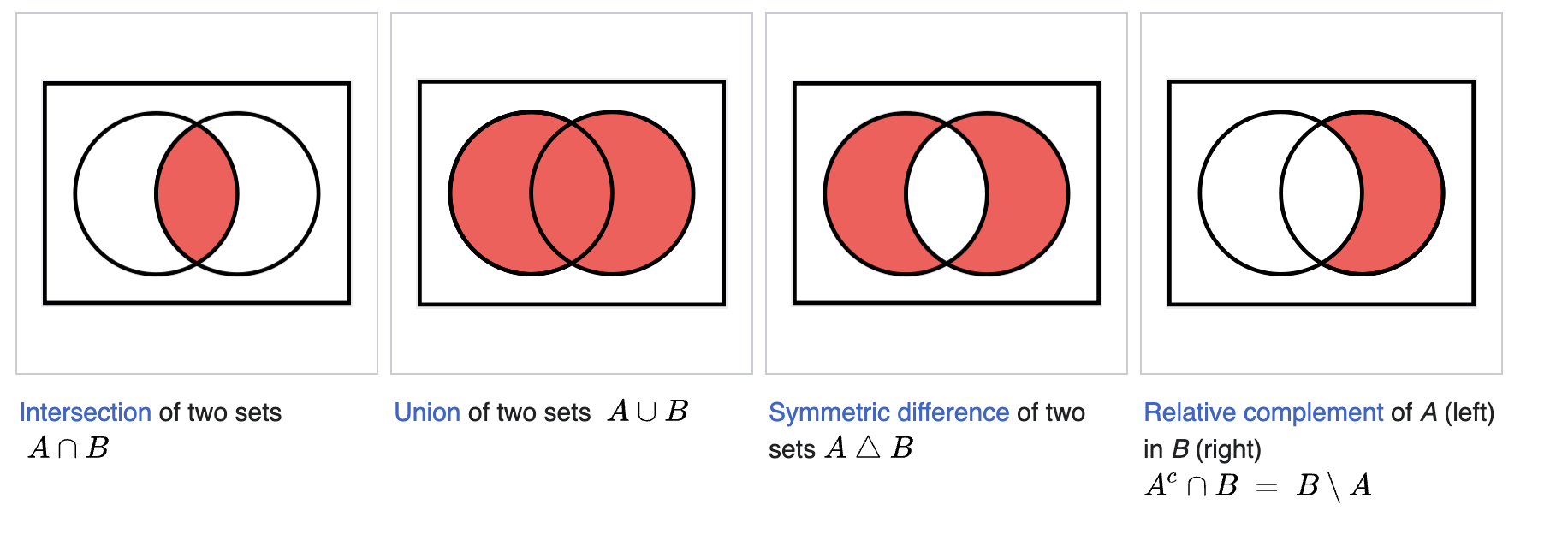
We can perform similar operations on 3D solids in KCL. They're sometimes called "3D booleans", because they perform the standard boolean set operations, but on 3D bodies. They're also known as "constructive solid geometry" operations (CSG) because they let you take existing solid geometory, and construct new geometries from them.
Let's see how these operations work. Here's two cubes.
// Sketch a square
sketch001 = sketch(on = XY) {
  // Sketch a rectangle first.
  line1 = line(start = [var -2.21mm, var -5.39mm], end = [var 2.8mm, var -5.39mm])
  line2 = line(start = [var 2.8mm, var -5.39mm], end = [var 2.8mm, var -0.39mm])
  line3 = line(start = [var 2.8mm, var -0.39mm], end = [var -2.21mm, var -0.39mm])
  line4 = line(start = [var -2.21mm, var -0.39mm], end = [var -2.21mm, var -5.39mm])
  coincident([line1.end, line2.start])
  coincident([line2.end, line3.start])
  coincident([line3.end, line4.start])
  coincident([line4.end, line1.start])
  parallel([line2, line4])
  parallel([line3, line1])
  perpendicular([line1, line2])
  horizontal(line3)

  // Make all sides the same length (i.e. make the rectangles square).
  distance([line1.start, line1.end]) == 5
  equalLength([line1, line2, line3, line4])
}

region001 = region(point = [0.295mm, -5.3875mm], sketch = sketch001)
cubeGreen = extrude(region001, length = 5)
  |> appearance(color = "#229922")

cubeBlue = clone(cubeGreen)
  |> translate(x = 3, z = 2, y = 1)
  |> appearance(color = "#222299")
union, intersect and subtract functions on these. Firstly, let's do a union. This should create a new solid which combines both input solids.
// This part is unchanged from previous examples.
sketch001 = sketch(on = XY) {
  line1 = line(start = [var -2.21mm, var -5.39mm], end = [var 2.8mm, var -5.39mm])
  line2 = line(start = [var 2.8mm, var -5.39mm], end = [var 2.8mm, var -0.39mm])
  line3 = line(start = [var 2.8mm, var -0.39mm], end = [var -2.21mm, var -0.39mm])
  line4 = line(start = [var -2.21mm, var -0.39mm], end = [var -2.21mm, var -5.39mm])
  coincident([line1.end, line2.start])
  coincident([line2.end, line3.start])
  coincident([line3.end, line4.start])
  coincident([line4.end, line1.start])
  parallel([line2, line4])
  parallel([line3, line1])
  perpendicular([line1, line2])
  horizontal(line3)
  distance([line1.start, line1.end]) == 5
  equalLength([line1, line2, line3, line4])
}

region001 = region(point = [0.295mm, -5.3875mm], sketch = sketch001)
cubeGreen = extrude(region001, length = 5)
  |> appearance(color = "#229922")
cubeBlue = clone(cubeGreen)
  |> translate(x = 3, z = 2, y = 1)
  |> appearance(color = "#222299")

// Apply a CSG operation.
both = union([cubeGreen, cubeBlue])
union of our two cubes has the exact same dimensions and position as the two cubes, but they've been combined into one solid body. The resulting solid inherits the green appearance of the first body in the union (if you swapped the order to [cubeBlue, cubeGreen] instead, the final solid would be blue).
What's the point of doing this? Now we can use transforms like appearance or rotate on the single unified solid. Previously we needed to transform each part separately, which can get annoying. Now that it's a single body, transformations will apply to the whole thing -- both the first cube's volume, and the second cube's.
Note: Instead of writing union([cubeGreen, cubeBlue]) you can use the shorthand cubeGreen + cubeBlue or cubeGreen | cubeBlue. This is a nice little shorthand you can use if you want to.
Let's try an intersection. This combines both cubes, but leaves only the volume from where they overlapped.
// This part is unchanged from previous examples.
sketch001 = sketch(on = XY) {
  line1 = line(start = [var -2.21mm, var -5.39mm], end = [var 2.8mm, var -5.39mm])
  line2 = line(start = [var 2.8mm, var -5.39mm], end = [var 2.8mm, var -0.39mm])
  line3 = line(start = [var 2.8mm, var -0.39mm], end = [var -2.21mm, var -0.39mm])
  line4 = line(start = [var -2.21mm, var -0.39mm], end = [var -2.21mm, var -5.39mm])
  coincident([line1.end, line2.start])
  coincident([line2.end, line3.start])
  coincident([line3.end, line4.start])
  coincident([line4.end, line1.start])
  parallel([line2, line4])
  parallel([line3, line1])
  perpendicular([line1, line2])
  horizontal(line3)
  distance([line1.start, line1.end]) == 5
  equalLength([line1, line2, line3, line4])
}

region001 = region(point = [0.295mm, -5.3875mm], sketch = sketch001)
cubeGreen = extrude(region001, length = 5)
  |> appearance(color = "#229922")
cubeBlue = clone(cubeGreen)
  |> translate(x = 3, z = 2, y = 1)
  |> appearance(color = "#222299")

// Apply a CSG operation.
both = intersect([cubeGreen, cubeBlue])
Note: Instead of writing intersect([cubeGreen, cubeBlue]) you can use the shorthand cubeGreen & cubeBlue. This is a nice little shorthand you can use if you want to.
Lastly, let's try a subtract call:
// This part is unchanged from previous examples.
sketch001 = sketch(on = XY) {
  line1 = line(start = [var -2.21mm, var -5.39mm], end = [var 2.8mm, var -5.39mm])
  line2 = line(start = [var 2.8mm, var -5.39mm], end = [var 2.8mm, var -0.39mm])
  line3 = line(start = [var 2.8mm, var -0.39mm], end = [var -2.21mm, var -0.39mm])
  line4 = line(start = [var -2.21mm, var -0.39mm], end = [var -2.21mm, var -5.39mm])
  coincident([line1.end, line2.start])
  coincident([line2.end, line3.start])
  coincident([line3.end, line4.start])
  coincident([line4.end, line1.start])
  parallel([line2, line4])
  parallel([line3, line1])
  perpendicular([line1, line2])
  horizontal(line3)
  distance([line1.start, line1.end]) == 5
  equalLength([line1, line2, line3, line4])
}

region001 = region(point = [0.295mm, -5.3875mm], sketch = sketch001)
cubeGreen = extrude(region001, length = 5)
  |> appearance(color = "#229922")
cubeBlue = clone(cubeGreen)
  |> translate(x = 3, z = 2, y = 1)
  |> appearance(color = "#222299")

// Apply a CSG operation.
both = subtract(cubeGreen, tools = [cubeBlue])
subtract is a little different. The first argument is the solid (or solids) which will have some volume carved out. The second argument is a list of solids to cut out. You can think of these as "tools" -- you're basically passing tools of various shapes which can carve out special volumes.
Let's try a subtraction with multiple tools:
// This part is unchanged from previous examples.
sketch001 = sketch(on = XY) {
  line1 = line(start = [var -2.21mm, var -5.39mm], end = [var 2.8mm, var -5.39mm])
  line2 = line(start = [var 2.8mm, var -5.39mm], end = [var 2.8mm, var -0.39mm])
  line3 = line(start = [var 2.8mm, var -0.39mm], end = [var -2.21mm, var -0.39mm])
  line4 = line(start = [var -2.21mm, var -0.39mm], end = [var -2.21mm, var -5.39mm])
  coincident([line1.end, line2.start])
  coincident([line2.end, line3.start])
  coincident([line3.end, line4.start])
  coincident([line4.end, line1.start])
  parallel([line2, line4])
  parallel([line3, line1])
  perpendicular([line1, line2])
  horizontal(line3)
  distance([line1.start, line1.end]) == 5
  equalLength([line1, line2, line3, line4])
}

region001 = region(point = [0.295mm, -5.3875mm], sketch = sketch001)
cubeGreen = extrude(region001, length = 5)
  |> appearance(color = "#229922")
cubeBlue = clone(cubeGreen)
  |> translate(x = 3, z = 2, y = 1)
  |> appearance(color = "#222299")


// Add another blue cube.
cubeBlue2 = clone(cubeBlue)
  |> translate(x = -6)

// Cut both blue cubes out of the green cube.
both = subtract(cubeGreen, tools = [cubeBlue, cubeBlue2])
// Sketch a square
sketch001 = sketch(on = XY) {
  // Sketch a rectangle first.
  line1 = line(start = [var -2.21mm, var -5.39mm], end = [var 2.8mm, var -5.39mm])
  line2 = line(start = [var 2.8mm, var -5.39mm], end = [var 2.8mm, var -0.39mm])
  line3 = line(start = [var 2.8mm, var -0.39mm], end = [var -2.21mm, var -0.39mm])
  line4 = line(start = [var -2.21mm, var -0.39mm], end = [var -2.21mm, var -5.39mm])
  coincident([line1.end, line2.start])
  coincident([line2.end, line3.start])
  coincident([line3.end, line4.start])
  coincident([line4.end, line1.start])
  parallel([line2, line4])
  parallel([line3, line1])
  perpendicular([line1, line2])
  horizontal(line3)

  // Make all sides the same length (i.e. make the rectangles square).
  distance([line1.start, line1.end]) == 5
  equalLength([line1, line2, line3, line4])
}
region001 = region(point = [0.295mm, -5.3875mm], sketch = sketch001)

// Target 1
cubeGreen = extrude(region001, length = 5)
  |> appearance(color = "#229922")

// Target 2
cubeGreen2 = clone(cubeGreen)
  |> translate(x = 6, y = 2)

// Tool
cubeBlue = clone(cubeGreen)
  |> translate(x = 3, z = 2, y = 1)
  |> appearance(color = "#222299")

// Do the subtraction
both = subtract([cubeGreen, cubeGreen2], tools = [cubeBlue])
// Sketch a square
sketch001 = sketch(on = XY) {
  // Sketch a rectangle first.
  line1 = line(start = [var -2.21mm, var -5.39mm], end = [var 2.8mm, var -5.39mm])
  line2 = line(start = [var 2.8mm, var -5.39mm], end = [var 2.8mm, var -0.39mm])
  line3 = line(start = [var 2.8mm, var -0.39mm], end = [var -2.21mm, var -0.39mm])
  line4 = line(start = [var -2.21mm, var -0.39mm], end = [var -2.21mm, var -5.39mm])
  coincident([line1.end, line2.start])
  coincident([line2.end, line3.start])
  coincident([line3.end, line4.start])
  coincident([line4.end, line1.start])
  parallel([line2, line4])
  parallel([line3, line1])
  perpendicular([line1, line2])
  horizontal(line3)

  // Make all sides the same length (i.e. make the rectangles square).
  distance([line1.start, line1.end]) == 5
  equalLength([line1, line2, line3, line4])
}
region001 = region(point = [0.295mm, -5.3875mm], sketch = sketch001)

// Make two green cubes and two blue cubes.
cubeGreen = extrude(region001, length = 5)
  |> appearance(color = "#229922")

cubeGreen2 = clone(cubeGreen)
  |> translate(x = 6, y = 2)

cubeBlue = clone(cubeGreen)
  |> translate(x = 3, z = 2, y = 1)
  |> appearance(color = "#222299")

cubeBlue2 = clone(cubeBlue)
  |> translate(x = -1, y = -4, z = -1)
  |> rotate(yaw = 40deg)

// Subtract both blue from both green.
both = subtract([cubeGreen, cubeGreen2], tools = [cubeBlue, cubeBlue2])
Advanced options
There's a few arguments you can set for these functions. To be honest, you probably won't ever need to set these manually, but they're documented here just in case.
toleranceis a measure of how accurate the underlying 3D combination algorithms are. A tolerance of0.1means the algorithm is very inaccurate, but very fast. A tolerance of0.000000001makes the algorithm much more accurate, but slower. This is set to a sensible default, but you might need to change it for models with very precise, very small features.legacyMethodlets you opt back into an older version of Zoo's geometry engine which used a different algorithm for CSG. We don't recommend setting this, and it will be removed at some point in the future.
Patterns
Real-world objects often have repeated parts. Consider a LEGO brick, which has a lot of repeated bumps on its top face. Or a table, with four repeated legs. KCL would be a very tedious language if we made you define each leg, or each LEGO bump, over and over again every time your model needed one. Luckily, there's a simple way to repeat geometry in your model. It's called a pattern. There are several ways to use patterns. Let's learn how they work!
Basic patterns
Let's start simple. We can use patterns to replicate our geometry, copying it into our scene several times. Let's take this simple cylinder, and copy it 4 times.
// Sketch a circle
circleSketch = sketch(on = XY) {
  circle1 = circle(start = [var -1mm, var 1mm], center = [var 0mm, var 0mm])
  coincident([circle1.center, ORIGIN])
  distance([circle1.start, circle1.center]) == 2mm
}

// Extrude it into a cylinder, then pattern it.
cylinders = extrude(region(sketch = circleSketch, point = [0, 0]), length = 4)
  |> patternLinear3d(instances = 4, distance = 10, axis = X)
patternLinear3d function takes 4 args:
- A solid to pattern (the unlabeled first arg, which is implicitly set to % and therefore gets the result of the
extrude()call, i.e. the cylinder, piped in) - The total number of instances you want (i.e. how many total copies of the solid there should be)
- How far apart each instance of the pattern should be
- The axis along which to place the copies.
In our above example, it places 3 extra instances (for a total of 4) along the X axis, each 10 units apart.
Note: You can choose a standard axis like X, Y or Z, but you can also use any vector as an axis, like [1, 1, 0.5].
Circular patterns
You can also use patterns to replicate something and lay them out in an arc around a point. We'll use the patternCircular3d function. Here's an example where we put 12 cubes in a circle:
// Sketch a square, just like normal.
sketch001 = sketch(on = XZ) {
  line1 = line(start = [var 2.66mm, var -2.08mm], end = [var -2.31mm, var -2.08mm])
  line2 = line(start = [var -2.31mm, var -2.08mm], end = [var -2.31mm, var 2.48mm])
  line3 = line(start = [var -2.31mm, var 2.48mm], end = [var 2.66mm, var 2.48mm])
  line4 = line(start = [var 2.66mm, var 2.48mm], end = [var 2.66mm, var -2.08mm])
  coincident([line1.end, line2.start])
  coincident([line2.end, line3.start])
  coincident([line3.end, line4.start])
  coincident([line4.end, line1.start])
  parallel([line2, line4])
  parallel([line3, line1])
  perpendicular([line1, line2])
  horizontal(line3)
  equalLength([line1, line2, line3, line4])
  distance([line2.start, line2.end]) == 5mm
  coincident([line3.start, ORIGIN])
}

// Extrude square into a cube.
region001 = region(point = [2.38mm, -4.7575mm], sketch = sketch001)
cube = extrude(region001, length = 5)

// First, move the square to the northernmost position (like 12 o'clock)
translate(cube, z = 30)

// Then pattern the cube 12 times, around the origin.
  |> patternCircular3d(
       instances = 12,
       axis = Y,
       center = [0, 0, 0],
       arcDegrees = 360deg,
       rotateDuplicates = false,
     )
[0, 0, 0]. We drew the first cube at the northernmost position (12 o'clock) and all the other instances were patterned around that center. Nice!
Note: The center argument is optional, and defaults to [0, 0, 0].
Notice that we used rotateDuplicates = false. If we set it to true, each duplicate object is also rotated as it is copied around the circle, so that they're all facing the center. Like this:
// Sketch a square.
sketch001 = sketch(on = XZ) {
  line1 = line(start = [var 2.66mm, var -2.08mm], end = [var -2.31mm, var -2.08mm])
  line2 = line(start = [var -2.31mm, var -2.08mm], end = [var -2.31mm, var 2.48mm])
  line3 = line(start = [var -2.31mm, var 2.48mm], end = [var 2.66mm, var 2.48mm])
  line4 = line(start = [var 2.66mm, var 2.48mm], end = [var 2.66mm, var -2.08mm])
  coincident([line1.end, line2.start])
  coincident([line2.end, line3.start])
  coincident([line3.end, line4.start])
  coincident([line4.end, line1.start])
  parallel([line2, line4])
  parallel([line3, line1])
  perpendicular([line1, line2])
  horizontal(line3)
  equalLength([line1, line2, line3, line4])
  distance([line2.start, line2.end]) == 5mm
  coincident([line3.start, ORIGIN])
}

// Extrude square into a cube.
region001 = region(point = [2.38mm, -4.7575mm], sketch = sketch001)
cube = extrude(region001, length = 5)

// First, move the square to the northernmost position (like 12 o'clock)
translate(cube, z = 30)
  // Then pattern the cube 12 times, around the origin.
  |> patternCircular3d(
       instances = 12,
       axis = Y,
       center = [0, 0, 0],
       arcDegrees = 360deg,
       rotateDuplicates = true,
     )
arcDegrees argument is optional, and defaults to 360 degrees. We can set it to 240deg to only pattern around two thirds of the circle instead:
// Sketch a square.
sketch001 = sketch(on = XZ) {
  line1 = line(start = [var 2.66mm, var -2.08mm], end = [var -2.31mm, var -2.08mm])
  line2 = line(start = [var -2.31mm, var -2.08mm], end = [var -2.31mm, var 2.48mm])
  line3 = line(start = [var -2.31mm, var 2.48mm], end = [var 2.66mm, var 2.48mm])
  line4 = line(start = [var 2.66mm, var 2.48mm], end = [var 2.66mm, var -2.08mm])
  coincident([line1.end, line2.start])
  coincident([line2.end, line3.start])
  coincident([line3.end, line4.start])
  coincident([line4.end, line1.start])
  parallel([line2, line4])
  parallel([line3, line1])
  perpendicular([line1, line2])
  horizontal(line3)
  equalLength([line1, line2, line3, line4])
  distance([line2.start, line2.end]) == 5mm
  coincident([line3.start, ORIGIN])
}

// Extrude square into a cube.
region001 = region(point = [2.38mm, -4.7575mm], sketch = sketch001)
cube = extrude(region001, length = 5)

// First, move the square to the northernmost position (like 12 o'clock)
translate(cube, z = 30)
  // Then pattern the cube 12 times, around the origin.
  |> patternCircular3d(
       instances = 12,
       axis = Y,
       center = [0, 0, 0],
       arcDegrees = 240deg,
       rotateDuplicates = true,
     )
// Sketch a big circle.
bigCircleSketch = sketch(on = XZ) {
  circle1 = circle(start = [var 0mm, var 10mm], center = [var 0mm, var 0mm])
  coincident([circle1.center, ORIGIN])
  vertical([circle1.center, circle1.start])
  distance([circle1.start, circle1.center]) == 10
}

// Extrude it into a "base".
bigCircle = region(sketch = bigCircleSketch, point = [0, 0])
base = extrude(bigCircle, length = 2)

// Start sketching a smaller circle on that base.
face001 = faceOf(base, face = END)
smallCircleSketch = sketch(on = face001) {
  circle1 = circle(start = [var -0.83mm, var 8.27mm], center = [var 0mm, var 7.79mm])
  vertical([circle1.center, ORIGIN])
  vertical([circle1.center, circle1.start])
}

// Extrude that circle into a small cylinder,
// then pattern it around.
region(point = [0mm, 7.3125mm], sketch = smallCircleSketch)
  |> extrude(length = 2)
  |> patternCircular3d(
       instances = 6,
       axis = Y,
       useOriginal = true,
     )
useOriginal = false, so the entire solid (original and new volume added via sketch-on-face-then-extrude) will be patterned. You can set useOriginal = true to only pattern the part added via sketch-on-face-then-extrude.
In other words, when useOriginal = false (the default), the total modified solid (made from a parent solid, and the modification) will be patterned around the global scene. When useOriginal = true, the modification will be patterned around the parent solid.
Transform patterns
Circular and linear patterns cover a lot of really common use-cases for mechanical engineers. But sometimes you want to do more complicated patterns, in more complicated shapes. We can't add a dedicated pattern function for every single shape our users can think of -- that would be almost unmaintainable (there are infinite possible shapes, after all). Instead, KCL has a powerful, flexible interface for patterning solids in any arrangement you can think of. It's called a transform pattern. They're created with the patternTransform function. It takes a familiar instances argument, which controls how many total copies of the shape you want. But it takes a new argument, called transform. This is a custom function. We'll dive deeper into those in the following chapters, but for now, they're basically just a way to calculate how to transform each replica in the pattern.
When might you need a pattern transform? Here's one use: to do a 2D pattern, like tiling a grid. Let's use a pattern transform to make a 5 by 5 grid.
numColumns = 5    // how many columns in our grid
width = 10        // side length of each square
gap = 1.5 * width // gap between each square

// Sketch a square
squareSketch = sketch(on = XY) {
  line1 = line(start = [var -1.35mm, var 1.51mm], end = [var 1.44mm, var 1.51mm])
  line2 = line(start = [var 1.44mm, var 1.51mm], end = [var 1.44mm, var -1.25mm])
  line3 = line(start = [var 1.44mm, var -1.25mm], end = [var -1.35mm, var -1.25mm])
  line4 = line(start = [var -1.35mm, var -1.25mm], end = [var -1.35mm, var 1.51mm])
  coincident([line1.end, line2.start])
  coincident([line2.end, line3.start])
  coincident([line3.end, line4.start])
  coincident([line4.end, line1.start])
  parallel([line2, line4])
  parallel([line3, line1])
  perpendicular([line1, line2])
  horizontal(line3)
  equalLength([line1, line2, line3, line4])
  distance([line4.start, line4.end]) == width
}

// Transform function.
// This takes in the instance number (called `i`), and returns a transform
// object that tells KCL how to transform that instance.
fn grid(@i) {
  column = rem(i, divisor = numColumns)
  row = floor(i / numColumns)
  // Return a KCL object, with one property, `translate`.
  // The `translate` property tells KCL how to translate each duplicated solid.
  return {
    translate = [column * gap, row * gap, 0]
  }
}

// Extrude square, then pattern it using the transform function.
region(point = [0.0450001mm, 5.1274998mm], sketch = squareSketch)
  |> extrude(length = 2)
  |> patternTransform(instances = numColumns * numColumns, transform = grid)
We've defined a custom function called grid. This function will get called once for every replica in the pattern, and it tells KCL how each replica should be transformed. Specifically it:
- Takes a single argument called
i. It's used to indicate which number replica is currently being processed. The first copy made will setito 1, the second copy will setito 2, etc. The argumentiis prefixed with@to indicate it's this function's special first unlabeled argument, so if you call it, you'd call it likegrid(1)orgrid(2), notgrid(i = 1). - Returns a list of different properties to transform in each replica.
In this example, we define a function grid which tells patternTransform to translate each replica by a certain amount column * gap along the X axis, row * gap along the Y axis, and to stay on the same location on the Z axis (i.e. move exactly 0 along that axis).
The grid function is called by patternTransform as many times as patternTransform's first argument, instances. On each call to grid the current instance number is passed and bound to i. In this example, because numColumns is 5 and the code uses instances = numColumns * numColumns, there will be 5 * 5 = 25 instances. So the pattern transform will call grid(0), grid(1) ... grid(24).
The specific value of row and column changes every time the grid function is called, because these variables are calculated from the input argument i. Remember, i represents which number replication we're transforming. To calculate column and row we're going to use a few new KCL functions we haven't seen before.
Firstly, rem. The value rem(i, divisor = n) will divide i by n and return the remainder. This means that for i = 0, 1, 2, 3, 4, x will equal 0, 1, 2, 3 and 4. But when i = 5 (i.e. the fifth copy is being calculated), x will be 0. We're calling this function 25 times, and over those calls, x will step from 0 to 4, jump back down to 0, and begin stepping up again. This means x is a good way to calculate the columns, which range from column 0 to column 4 (a total of 5 columns).
The floor function takes a fractional number, and rounds it down to the nearest integer. For example, floor(3.6) is 3. This means it's a good way to calculate the row, because the first five times it's called, row will always equal 0. It'll round down (i / n) from 0/5, 1/5, 2/5, 3/5, 4/5 all down to 0. Then the sixth time it's called, it will receive 5/5, which is 1, and round it down to 1. These neat little mathematical tricks mean we can calculate the row and column from the repetition number i.
The final result speaks for itself:
numColumns = 5    // how many columns in our grid
width = 10        // side length of each square
gap = 1.05 * width // gap between each square

// Sketch a square
squareSketch = sketch(on = XY) {
  line1 = line(start = [var -1.35mm, var 1.51mm], end = [var 1.44mm, var 1.51mm])
  line2 = line(start = [var 1.44mm, var 1.51mm], end = [var 1.44mm, var -1.25mm])
  line3 = line(start = [var 1.44mm, var -1.25mm], end = [var -1.35mm, var -1.25mm])
  line4 = line(start = [var -1.35mm, var -1.25mm], end = [var -1.35mm, var 1.51mm])
  coincident([line1.end, line2.start])
  coincident([line2.end, line3.start])
  coincident([line3.end, line4.start])
  coincident([line4.end, line1.start])
  parallel([line2, line4])
  parallel([line3, line1])
  perpendicular([line1, line2])
  horizontal(line3)
  equalLength([line1, line2, line3, line4])
  distance([line4.start, line4.end]) == width
}

// Transform function
fn grid(@i) {
  column = rem(i, divisor = numColumns)
  row = floor(i / numColumns)
  // Is `i` an even, or odd, number?
  isEven = rem(i, divisor = 2) == 0

  return {
    translate = [column * gap, row * gap, 0],
    // Only create a replica if `isEven` is true.
    replicate = isEven,
  }
}

// Extrude square, then pattern it using the transform function.
region(point = [0.0450001mm, 5.1274998mm], sketch = squareSketch)
  |> extrude(length = 2)
  |> patternTransform(instances = numColumns * numColumns, transform = grid)
In this example, we use a very similar transform function. The only difference is, we're setting the replicate property on the final transform too. And we're setting it to the variable isEven. This variable is a boolean value -- it's true if i divided by 2 has a remainder of 0, which is the definition of an even number (it's divisible by 2). This should skip every second replication. Let's try it out!
width = 10        // side length of each square

// Sketch a square
squareSketch = sketch(on = XY) {
  line1 = line(start = [var -1.35mm, var 1.51mm], end = [var 1.44mm, var 1.51mm])
  line2 = line(start = [var 1.44mm, var 1.51mm], end = [var 1.44mm, var -1.25mm])
  line3 = line(start = [var 1.44mm, var -1.25mm], end = [var -1.35mm, var -1.25mm])
  line4 = line(start = [var -1.35mm, var -1.25mm], end = [var -1.35mm, var 1.51mm])
  coincident([line1.end, line2.start])
  coincident([line2.end, line3.start])
  coincident([line3.end, line4.start])
  coincident([line4.end, line1.start])
  parallel([line2, line4])
  parallel([line3, line1])
  perpendicular([line1, line2])
  horizontal(line3)
  equalLength([line1, line2, line3, line4])
  distance([line4.start, line4.end]) == width
}

fn transform(@i) {
  return {
    // Move down each time.
    translate = [0, 0, -i * width],
    // Make the cube longer, wider and flatter each time.
    scale = [
      pow(1.1, exp = i),
      pow(1.1, exp = i),
      pow(0.9, exp = i)
    ],
    // Turn by 15 degrees each time.
    rotation = { angle = 15 * i, origin = "local" }
  }
}


// Extrude square, then pattern it using the transform function.
region(point = [0.0450001mm, 5.1274998mm], sketch = squareSketch)
  |> extrude(length = 2)
  |> patternTransform(instances = 25, transform)
In this example, we make 25 cubes, slightly transforming each one. Each cube gets translated (moving down along the Z axis), and scaled (becoming longer, wider and flatter), as well as rotating 15 degrees around its own center (i.e. its local origin). We could rotate them around the scene's center by using origin = "global". Here's the result.
Pattern transforms are a very powerful tool. They're definitely one of the most complex function in KCL, but that complexity gives you a lot of flexibility. Any mathematical curve you can formulate can be used to pattern your instances, by just calculating it in a transform function. The same goes for tiling or grid arrangements. For more examples, you can read the full patternTransform docs.
2D patterns and holes
WARNING: 2D patterns are, currently, only supported for our old sketch syntax. We're actively working on porting 2D patterns to our new sketch syntax, so you can use them with constraint solvers. Until then, you can read the rest of this chapter and use it with our old sketch syntax.
So far all of the patterns we've used have replicated 3D solids. But you can use patterns to replicate 2D sketches too. The patternLinear2d, patternCircular2d and patternTransform2d functions work like their 3D variants, except they take 2D axes and 2D points. Here's a simple example:
manyCircles = startSketchOn(XZ)
  |> circle(radius = 4, center = [50, 0])
  |> patternCircular2d(
       center = [0, 0],
       instances = 12,
       arcDegrees = 360deg,
       rotateDuplicates = true,
     )
extrude(manyCircles, length = 10) to the end of the above KCL program. But it's not a good idea, because it produces the exact same model as you would have gotten from making a single 3D solid, then using 3D patterns on that. The only difference is, extruding a 2D pattern is much slower than patterning a 3D solid. So, can we do anything useful with 2D patterns?
Yes! One important use case is putting holes into 2D sketches. We have a special subtract2d function for this. Let's take the pattern from above, and use it to cut holes into another sketch.
manyCircles = startSketchOn(XZ)
  |> circle(radius = 4, center = [50, 0])
  |> patternCircular2d(
       center = [0, 0],
       instances = 12,
       arcDegrees = 360deg,
       rotateDuplicates = true,
     )

base = startSketchOn(XZ)
  |> circle(radius = 60, center = [0, 0])
  |> subtract2d(tool = manyCircles)
  |> extrude(length = 10)
subtract2d, you should consider it.
Functions and parametric design
In mechanical engineering, parametric design is a key tool that helps you avoid redundant work when you're designing the same object over and over again with slight tweaks. In software engineering, functions are a key tool that help you avoid redundant work when you're designing the same software over and over again with slight tweaks.
That's right -- breaking a mechanical engineering project into several key parametric designs is basically the same as breaking a software engineering project into several key functions. KCL makes parametric design easy and convenient with functions. You'll declare functions to represent parametric designs, and you'll call those functions with specific arguments to produce specific designs with the right parameters. Let's see how.
Function declaration
We briefly looked at function declarations when we covered pattern transforms. Let's write an example function declaration and analyze its parts.
fn add(a, b) {
  sum = a + b
  return sum
}
A function declaration has a few key parts. Let's look at each one, in the order they appear:
- The
fnkeyword - The function's name
- Round parentheses
(and) - Within those parentheses, a list of argument names
- Curly brackets
{and} - Within those brackets, KCL code, which may end with a
returnstatement.
This function takes two arguments, a and b, adds them, and returns their sum as the function's output. When a function executes the return statement, it evaluates the expression after return, stops executing, and outputs that value. You can call our example function like this:
sum = add(a = 1, b = 2)
Functions can also declare one unlabeled arg. If you do want to declare an unlabeled arg, it must be the first arg declared. When declaring an unlabeled arg, prefix it with @, like here:
// The @ indicates an argument can be used without a label.
// Note that only the first argument can use @.
fn increment(@x) {
  return x + 1
}

fn add(@x, delta) {
  return x + delta
}

two = increment(1)
three = add(1, delta = 2)
Mechanical engineering with functions
Let's use functions to build a parametric pipe flange. We can start with a specific design, with specific direct measurements. Then we'll learn how to parameterize it. Then we can easily make a lot of similar pipe flanges with different parameters.
Here's a specific model. It's got 8 unthreaded holes, each with a radius of 4, and the overall model has a radius of 60. It's 10mm thick.
// Sketch a big circle.
bigCircleSketch = sketch(on = XZ) {
  circle1 = circle(start = [var 0mm, var 10mm], center = [var 0mm, var 0mm])
  coincident([circle1.center, ORIGIN])
  vertical([circle1.center, circle1.start])
  distance([circle1.start, circle1.center]) == 60
}

// Extrude it into a "base".
bigCircle = region(sketch = bigCircleSketch, point = [0, 0])
thickness = 10mm
base = extrude(bigCircle, length = thickness, symmetric = true)

// Start sketching a smaller circle
smallCircleSketch = sketch(on = XZ) {
  circle1 = circle(start = [var -0.83mm, var 8.27mm], center = [var 0mm, var 7.79mm])
  vertical([circle1.center, ORIGIN])
  vertical([circle1.center, circle1.start])
  distance([circle1.start, circle1.center]) == 4
}

// Extrude that circle into a small cylinder,
// then pattern it around, making little pegs.
pegs = region(point = [0mm, 7.3125mm], sketch = smallCircleSketch)
  |> extrude(length = thickness * 3, symmetric = true)
  |> translate(x = 50)
  |> patternCircular3d(instances = 8, axis = Y, useOriginal = true)

// Remove the pegs from the base.
baseWithHoles = subtract(base, tools = pegs)
flange which takes in several parameters. Let's see:
// Define a parametric flange
fn flange(numHoles, holeRadius, baseRadius, thickness, holeEdgeGap) {
  // Sketch a big circle.
  bigCircleSketch = sketch(on = XZ) {
    circle1 = circle(start = [var 0mm, var 10mm], center = [var 0mm, var 0mm])
    coincident([circle1.center, ORIGIN])
    vertical([circle1.center, circle1.start])
    distance([circle1.start, circle1.center]) == baseRadius
  }

  // Extrude it into a "base".
  bigCircle = region(sketch = bigCircleSketch, point = [0, 0])
  base = extrude(bigCircle, length = thickness, symmetric = true)

  // Start sketching a smaller circle
  smallCircleSketch = sketch(on = XZ) {
    circle1 = circle(start = [var -0.83mm, var 8.27mm], center = [var 0mm, var 7.79mm])
    vertical([circle1.center, ORIGIN])
    vertical([circle1.center, circle1.start])
    distance([circle1.start, circle1.center]) == holeRadius
  }

  // Extrude that circle into a small cylinder,
  // then pattern it around, making little pegs.
  pegs = region(point = [0mm, 7.3125mm], sketch = smallCircleSketch)
    |> extrude(length = thickness * 3, symmetric = true)
    |> translate(x = baseRadius - holeEdgeGap)
    |> patternCircular3d(instances = numHoles, axis = Y, useOriginal = true)

  // Remove the pegs from the base.
  return subtract(base, tools = pegs)
}

// Call our parametric flange function, passing in specific parameter values, to make a specific flange.
originalFlangeAgain = flange(
  numHoles = 8,
  holeRadius = 5,
  baseRadius = 60,
  thickness = 10,
  holeEdgeGap = 10,
)
First we defined a function for making a parametric flange. This lets us make many possible flanges. First, we made our original flange again. But we can also make a range of other flanges, by varying the parameters! Here's one:
flange(
  numHoles = 4,
  holeRadius = 15,
  baseRadius = 60,
  thickness = 20,
  holeEdgeGap = 20,
)
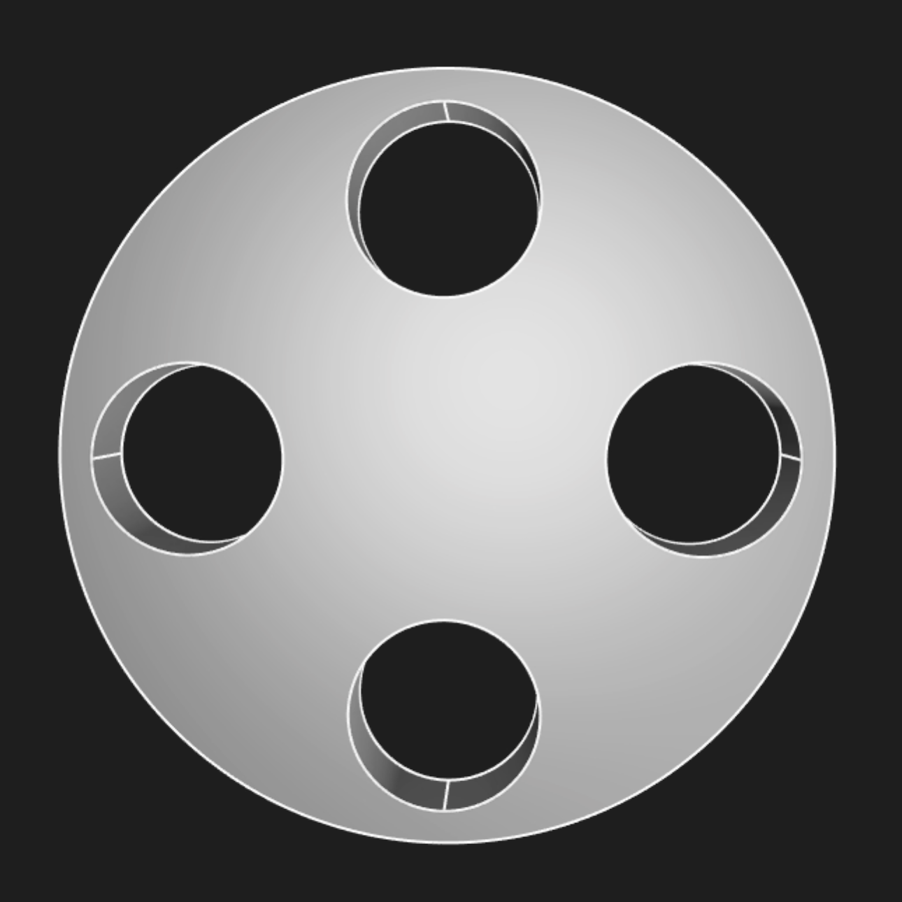
And let's try one more:
flange(
  numHoles = 20,
  holeRadius = 3,
  baseRadius = 90,
  thickness = 20,
  holeEdgeGap = 15,
)
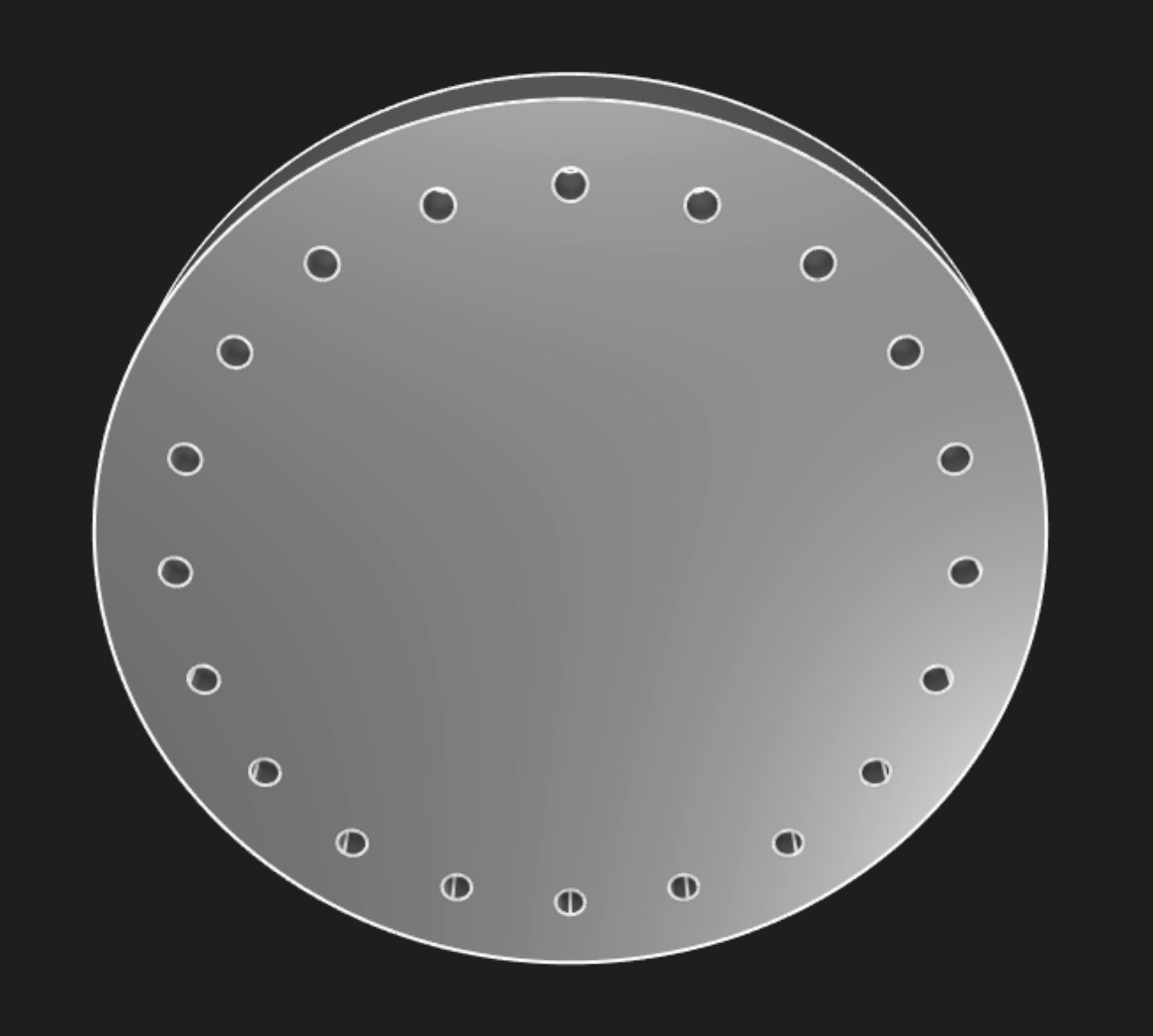
Replacing specific KCL code for a specific design with a parametric function gives you the flexibility to generate a lot of very similar designs, varying their parameters by passing in different arguments to suit whatever your project's requirements are.
Repeating geometry with functions
Functions can also be used to avoid writing the same code over and over again, in a single model. Sketch blocks can be quite long, because each constraint is typically on its own line, and complex models have a lot of constraints. Even just drawing a simple cube takes 16 lines of code: 4 to create lines, 4 to join those lines together via coincident constraints, and then 8 more to make the quadrilateral into a square of the chosen side length.
If we wanted to make 3 cubes, we shouldn't copy and paste this code 3 times. That would be annoying to read. We could use the clone() function to copy the cube, and then use transform functions like translate() or appearance() to tweak the cube. But we could also make a reusable cube helper function, like this.
/// Helper function to make a 3D cube with the given length and position along X.
fn cube(sideLen, offset) {
  sketch001 = sketch(on = XY) {
    line1 = line(start = [var 0mm, var 0mm], end = [var 3.08mm, var 0mm])
    line2 = line(start = [var 3.08mm, var 0mm], end = [var 3.08mm, var -3.01mm])
    line3 = line(start = [var 3.08mm, var -3.01mm], end = [var 0mm, var -3.01mm])
    line4 = line(start = [var 0mm, var -3.01mm], end = [var 0mm, var 0mm])
    coincident([line1.end, line2.start])
    coincident([line2.end, line3.start])
    coincident([line3.end, line4.start])
    coincident([line4.end, line1.start])
    parallel([line2, line4])
    parallel([line3, line1])
    perpendicular([line1, line2])
    horizontal(line3)
    coincident([line1.start, ORIGIN])
    equalLength([line1, line2, line3, line4])
    fixed([line1.start, ORIGIN])
    distance([line1.start, line1.end]) == sideLen
  }
  hide(sketch001)
  return region(sketch = sketch001, point = [0.4, -0.4])
    |> extrude(length = sideLen)
    |> translate(x = offset)
}

// Make two cubes, first one:
cube(sideLen = 2, offset = 2)
  |> appearance(color = "#26b8ba", metalness = 70, roughness = 40)

// And the second one:
cube(sideLen = 1, offset = 5)
  |> appearance(color = "#d205e1", metalness = 70, roughness = 40)
clone() and translate(). If we wanted to, say, tweak the height of each cube, we could add a new parameter height to our cube function. Or we could just alter the extrude length in the function body.
By putting the details of "what does a cube look like" in a single function, we make our code both more readable, and easier to change in the future.
Note: Currently, Zoo Design Studio doesn't support using point-and-click UI to change geometry created in functions. That's something we hope to support in the future.
Iterating with map and reduce
Every programming language has a way to do iteration: to repeat the same task many times. Traditional programming languages like Python, JavaScript or C use loops. KCL doesn't have any loops, but we have something very similar: arrays, and two helper functions called map and reduce. Let's see how they can solve problems.
Transforming arrays with map
The map function lets you transform an array by calling a function on every element. For example:
inputArray = [1, 2, 3, 4]
fn squareNumber(@x) { return x * x }
outputArray = map(inputArray, f = squareNumber)
The map function takes an input array as its first argument, then a function (its label is abbreviated to just f). It calls the function on every element of the input array, and returns it. If you open the Variables pane, you'll see that outputArray is [1, 4, 9, 16], just as we expected.
You can use map to create geometry too! For example, let's make 3 cubes, next to each other.
fn cube(@offset) {
  sideLen = 10
  sketch001 = sketch(on = XY) {
    line1 = line(start = [var 0mm, var 0mm], end = [var 3.08mm, var 0mm])
    line2 = line(start = [var 3.08mm, var 0mm], end = [var 3.08mm, var -3.01mm])
    line3 = line(start = [var 3.08mm, var -3.01mm], end = [var 0mm, var -3.01mm])
    line4 = line(start = [var 0mm, var -3.01mm], end = [var 0mm, var 0mm])
    coincident([line1.end, line2.start])
    coincident([line2.end, line3.start])
    coincident([line3.end, line4.start])
    coincident([line4.end, line1.start])
    parallel([line2, line4])
    parallel([line3, line1])
    perpendicular([line1, line2])
    horizontal(line3)
    coincident([line1.start, ORIGIN])
    equalLength([line1, line2, line3, line4])
    fixed([line1.start, ORIGIN])
    distance([line1.start, line1.end]) == sideLen
  }
  hide(sketch001)
  return region(sketch = sketch001, point = [0.4, -0.4])
    |> extrude(length = sideLen)
    |> translate(x = offset)
}

offsets = [0, 25, 50]
cubes = map(offsets, f = cube)
cube function on each offset in the array. The final result is an array of cubes. Calling the cube function drew the three cubes, each at their own offset.
So far so good. But this is basically just a 3D pattern. We can make this more interesting by making each cube a different color. Instead of an array of offsets, we'll store an array of offsets and colors. To do this, we'll make a KCL object. An object has multiple properties, each with its own label and value. For example:
myObject = {
  offset = 25,
  color = "#00ff00",
}
This object has two fields, offset and color. You could access them by calling myObject.offset and myObject.color. Let's see how we can use this with map:
fn cube(@params) {
  offset = params.x
  color = params.color
  sideLen = 10
  sketch001 = sketch(on = XY) {
    line1 = line(start = [var 0mm, var 0mm], end = [var 3.08mm, var 0mm])
    line2 = line(start = [var 3.08mm, var 0mm], end = [var 3.08mm, var -3.01mm])
    line3 = line(start = [var 3.08mm, var -3.01mm], end = [var 0mm, var -3.01mm])
    line4 = line(start = [var 0mm, var -3.01mm], end = [var 0mm, var 0mm])
    coincident([line1.end, line2.start])
    coincident([line2.end, line3.start])
    coincident([line3.end, line4.start])
    coincident([line4.end, line1.start])
    parallel([line2, line4])
    parallel([line3, line1])
    perpendicular([line1, line2])
    horizontal(line3)
    coincident([line1.start, ORIGIN])
    equalLength([line1, line2, line3, line4])
    fixed([line1.start, ORIGIN])
    distance([line1.start, line1.end]) == sideLen
  }
  hide(sketch001)
  return region(sketch = sketch001, point = [0.4, -0.4])
    |> extrude(length = sideLen)
    |> translate(x = offset)
    |> appearance(color = color)
}

offsets = [
  { x = 0, color = "#99ff99" },
  { x = 25, color = "#00ff00" },
  { x = 50, color = "#002200" }
]

threeCubes = map(offsets, f = cube)
map takes in an array, and outputs an array. The arrays always have the same length. Item x in the input array will be f(x) in the output array, where f is whichever function you pass in.
Anonymous functions
It can get annoying defining a new function every time you want to use map. For instance, in the earlier example where we defined a fn squareNumber to use in a map -- is that really necessary? If you have a lot of map calls, you'll slowly find your code becoming littered with tiny functions that you only use in a map.
KCL supports a nice little feature that can simplify this: anonymous functions. They're functions that don't have a name. You declare them where you need them, they're passed into mapand they aren't available after. Let's have a look:
inputArray = [1, 2, 3, 4]
outputArray = map(inputArray, f = fn (@x) { return x * x })
In this variation, we're passing in an anonymous function as the argument f of map. Just like before, it takes a single input argument x, squares it, and returns it. It should produce the exact same output as the earlier example with a function named squareNumber.
You can choose to use either named or anonymous functions with map. Neither is better or worse, you can use whichever you prefer. Generally, if a function is only a single line long, and you're only going to call it once (in a map or something similar), then you should consider making it anonymous and passing it as an argument directly.
Consuming arrays with reduce
The map function lets you iterate over an array, producing another array with the same length. But what if you don't want to get an array out? For example, what if you want to sum an array, or find the average?
The answer is: use the reduce function. This function, like map, takes an array and a function, then it calls the function on every element in the array. The difference is:
- In
map, the function argumentftakes a single arg: the array's item being processed, often calledi. - In
reduce, the function argumentftakes two args: the array's item being processedias well as a second value that accumulates across the array. It's calledaccum, short for reduce.
Let's see an example:
inputArray = [1, 2, 3, 4]
sum = reduce(inputArray, initial = 0, f = fn(@i, accum) { return i + accum })
If you open sum in the Variables pane, you'll see it's 10, as we expect. How does this work? Let's break it down and see what happens in each step of the reduce.
- The
reducestarts. It setsaccumto its initial value, which is theinitial = 0arg. So,accumstarts at 0. - Reduce starts iterating over the array.
- The first item is
1. Reduce callsf, passingi=1andaccum=0. Thenfreturns1+0, or 1. This becomes the new value ofaccum. - The next item is
2. Reduce callsf, passingi=2andaccum=1. Thenfreturns2+1, or 3. This becomes the new value ofaccum. - The next item is
3. Reduce callsf, passingi=3andaccum=3. Thenfreturns3+3, or 6. This becomes the new value ofaccum. - The next item is
4. Reduce callsf, passingi=4andaccum=6. Thenfreturns4+6, or 10. This becomes the new value ofaccum. - There's no more array items to handle, so reduce returns the last accumulated value, 10.
That's how reduce can take a long list of items and reduce it to a single item, accumulating the answer as it goes through the array.
What are some other things we can do with reduce? We could calculate the product of an array:
reduce(inputArray, initial = 1, f = fn(@i, accum) { return i * accum})
You'll find map and reduce useful when building geometry procedurally. They're useful programming primitives for building complex programs. It's important to check your work when you're writing code like this, that manipulates values like numbers and arrays, which can't be visualized like KCL sketches or solid geometry. In the next chapter, we'll learn how to check your work and write basic tests in KCL.
Checking your work
Correctness matters a lot in engineering. KCL tries to give you the tools you need to check your own work, and make sure your designs do exactly what you expect. In this chapter we'll explore ways to verify your KCL code does what you intended it to do.
Querying calculations
We've already covered this one, so I'll keep this brief. If you want to double-check your calculations, you can always assign some intermediate value to a variable, then view its value in the Variables panel in Zoo Design Studio. We saw an example of this earlier, where we broke up the quadratic equation into parts and inspected them. You can break complicated calculations into smaller parts, storing them in variables so they can be inspected individually.
Querying geometry
You can also query distances and angles, by measuring them with tags. Then you can assign those values to variables and read them off the Variables panel. We covered this previously, so refer back to that link for more detail.
Comments
Putting a comment in your code helps explain why you're doing something. Why was this edge double the size of the previous edge? Why was this particular curvature or angle chosen? Leaving comments in your code, like // Edge must be 1cm longer than front edge to accommodate button, helps explain to your colleagues why a certain decision was made. That way, when someone revisits the design in the future, they know if your original assumptions still hold, or if they can be changed.
Asserts
KCL's assert function lets you check that a certain variable has the expected value. In other words, you're asserting that the variable actually has the value you expect. If this assertion is wrong, KCL will stop executing and explain why. For example, let's add asserts to our quadratic equation calculations. We can calculate that the quadratic 2x^2 + 3x + 1 should have roots -0.5 and -1. Let's calculate it, and asserts to make sure we got the calculations correct.
// Coefficients that define the quadratic
a = 2
b = 3
c = 1

delta = pow(b, exp = 2) - (4 * a * c)
x0 = ((-b) + sqrt(delta)) / (2 * a)
x1 = ((-b) - sqrt(delta)) / (2 * a)

// Assert the two roots are what we expect.
assert(x0, isEqualTo = -0.5)
assert(x1, isEqualTo = -1)
This program was written correctly, so the KCL program runs just fine. But let's pretend we made a typo. We'll change c = 1 to c = 0, and rerun the program. You'll see the assert has an error now: "assert failed: Expected 0 to be equal to -0.5 but it wasn't".
Asserts work pretty similarly to looking up a variable in the Variables panel. Both let you check a value is what you expect. But asserts have two big advantages over checking the Variables panel.
Firstly, asserts are automatic. You can add asserts to your KCL code, and then every time the program runs, the asserts will get checked. You don't have to remember which values need checking. If you send your KCL file to a coworker, you don't have to explain "Hey, make sure to check that maximumStress is 1.25". You can just add the assert to your code, and all your coworkers will benefit from having the assertion checked. This is especially helpful for iterating on your design. You can start your design work by adding some asserts to check key requirements, and then as you keep tweaking and improving your design, KCL will automatically run all the asserts, and make sure the same properties are always checked.
Secondly, asserts are more flexible. You can check many different properties besides just checking two numbers are equal. For example, you can compare them and check if one number is greater or less than your variable:
wallMountingHoleDiameter = .625
wallMountLength = 2.25
assert(wallMountLength, isGreaterThanOrEqual = wallMountingHoleDiameter * 3)
You can add custom error messages to explain why this assertion is important:
wallMountingHoleDiameter = .625
wallMountLength = 2.25
assert(wallMountLength, isGreaterThanOrEqual = wallMountingHoleDiameter * 3, error = "This doesn't leave enough room for a hole. Either decrease hole diameter or increase wallMountLength")
You can also add a tolerance to your equality checks, to ensure that tiny little differences caused by floating-point math or approximation calculations don't trigger the error.
assert(1.0000001214, isEqualTo = 1.0, tolerance = 0.001)
Asserts and parametric design
For a realistic example of asserts, see this bracket we modelled in KCL. You can see the mechanical engineer designed this parametrically. They designed the bracket in terms of parameters like width, p (the force on the shelf), shelfMountLength etc. From these initial parameters, they calculate other quantities, like the moment or the thickness. Then they use asserts to make sure that when the parameters are changed, the results are still sensible. For example, they check that the parameters leave enough of a gap between the holes and the bracket's edge. They're also checking that the bracket is strong enough, by checking the actual stress on the model for these parameters (actualSigma) is below the maximum allowed stress, via assert(actualSigma, isLessThanOrEqual = sigmaAllow).
We could add more detailed checks by asserting that the parameters meet basic logical requirements -- for example, the width must be greater than zero to be meaningful. So you could add assert(width, isGreaterThan = 0).
By adding these asserts and comments, your CAD files become self-documenting. You don't need to email a PDF to your colleagues explaining why you chose the parameters you chose, or why certain lengths are they way they are. Your assertions both indicate what measurements or properties are important, and prove that your design has those important properties.
Summary
KCL helps you automatically check your work. You should be able to analyze your engineering designs as early as possible in the design process -- ideally, within Zoo Design Studio, long before you send the part away for manufacturing or analysis. You can check your work in the Variables panel, but we recommend adding assert statements to your KCL. You can use asserts to:
- Double-check your calculations, especially when transcribing engineering calculations into KCL
- Validate parameters in parametric design, like ensuring a radius or length is positive
- Check that your part fulfills its requirements, for example by calculating the maximum force it can tolerate, and asserting that maximum force is above your required minimum
- Query geometry like the angle between two lines with
segAngand ensure it's what you expect - Clearly explain what important requirements your design has, and how to correct mistakes if the assertion fails.
Types and Units
KCL tracks the type of each variable, and can help you avoid bugs by noticing when your types don't match. You may have noticed the very basic type checking already, for example trying to run 3 * true will cause an error. But KCL supports more helpful type checks. Let's see how!
Function signatures
Consider this KCL example.
// Could take either two strings, or two numbers.
fn makeMessage(prefix, suffix) {
  return prefix + suffix
}

msg1 = makeMessage(prefix = "hello", suffix = " world")
msg2 = makeMessage(prefix = 1, suffix = 3)
In this example, makeMessage takes two arguments and adds them together with +. If the two arguments are both strings, like in msg1, this will produce one concatenated string (like "hello world"). If the two args are numbers (like in msg2) this will add them together (in the example, producing 4).
This might not be the goal, though! Maybe you designed makeMessage to only work with numbers, or only work with strings. You can add a type to the argument, and KCL will make sure it's only called with those arguments. Like this:
// Note the types of arguments are given now.
fn makeMessage(prefix: string, suffix: string) {
  return prefix + suffix
}

msg1 = makeMessage(prefix = "hello", suffix = " world")
msg2 = makeMessage(prefix = 1, suffix = 3)
In this example, msg1 is defined successfully as "hello world", but KCL will exit with an error while running msg2, because the arguments being passed to it don't match the types the function declares.
Units of measurement
KCL tracks the units that each distance uses. This can help you accurately translate your engineering requirements or formula into KCL, without pulling out a calculator to convert between inches and centimeters.
For example, you can put a unit like 2cm or 2mm as the length of a line. Here's three different lines of length 20 centimeters, inches and millimeters.
sketch001 = sketch(on = XY) {
  line1 = line(start = [var -13.35mm, var 10.75mm], end = [var 10.94mm, var 10.42mm])
  line2 = line(start = [var -18.82mm, var 17.12mm], end = [var 25.39mm, var 11.53mm])
  line3 = line(start = [var -25.48mm, var 24.01mm], end = [var 35.37mm, var 17.12mm])
  distance([line3.start, line3.end]) == 2mm
  distance([line2.start, line2.end]) == 2cm
  distance([line1.start, line1.end]) == 2in
  parallel([line1, line2, line3])
}

Other suffixes include metres (m), feet (ft) and yards (yd).
In the previous examples, before this chapter, we always used general-purpose numbers with no units (like length = 20). Each KCL file has a default unit. You can set it by adding @settings(defaultLengthUnit = in) at the top of your KCL file. It has to go at the very top, before any code (although comments are permitted before it). If you don't set the default in @settings, your user- or project-level settings might set it. Otherwise, if you truly don't set anything, it'll default to millimeters.
You can also set the units for angle measurements. For example, you can revolve a sketch either 180deg or 3.14rad.
Mixing units
When you're doing arithmetic in KCL, you can mix and match numbers:
y = 3cm // roughly 1.18 inches
x = 10in - y
If you open the Variables pane, you'll see that x is 8.818 inches. KCL can track the numbers and types involved, letting you flexibly compare different units. However, KCL is not perfect at this (yet -- we're working on it!) For example, right now, KCL cannot anticipate what 30 inches multiplied by 2 centimeters is. If you try 30in * 2cm, you'll get a warning: Multiplying numbers which have unknown or incompatible units. KCL warns you so that you can explicitly provide units if you want.
// This causes a warning that KCL doesn't know what units `z` uses
z = 10in * 3cm
Units and function signatures
You can combine units of measurement and types! There are 3 kinds of number type:
- A specific unit, like
number(mm)ornumber(deg). - Some kind of number, like
number(Length), which accepts centimeters or inches, but not degrees or radians. Similarly,number(Angle)accepts degrees or radians, but not centimeters or inches. - Any kind of number, i.e. just
number.
These can be used in function signatures. If you define a function that accepts, say, centimeters, and someone passes in inches, the inches will automatically be converted to centimeters. This works just like the above example of 10in - 3cm, with the same limitations (sometimes you'll need to provide the type, like x: number(cm)).
Here's a user-defined function f that accepts some angle -- either degrees or radians, but not centimeters (which is a length, not an angle).
fn f(theta: number(Angle)) {
  return cos(theta)
}

xArg = 360deg
x = f(theta = xArg)
yArg = (2 * PI): number(rad)
y = f(theta = yArg)
If you try to run f(theta = 2in) you'll see an error that explains you're using the wrong type of number. But both x and y will correctly be 1 if you open the Variables panel, showing that their units are being tracked correctly.
Other types
Arrays and functions have their own type. You can look up these details at the types page in our docs.
Modules
So far, all the KCL examples we've seen have been fairly small. But as you start modeling larger projects, you'll find that your code no longer neatly fits into one file. Organizing your code into smaller modules can really help. In this chapter, we'll explain how to break your code into smaller modules, which let you break your one big KCL file into several smaller ones. This can help your models render much faster, by executing different modules in parallel.
Splitting code into modules
So far, all our KCL examples have been a single file -- main.kcl. That's the default name that Zoo Design Studio and other KCL tools (like our command-line interface) use. But what happens when main.kcl gets too big?
Say we have a KCL file like this, which defines a cube function, a sphere function, and then models several cubes and spheres.
fn cube() {
  sideLen = 10
  sketch001 = sketch(on = XY) {
    line1 = line(start = [var 0mm, var 0mm], end = [var 3.08mm, var 0mm])
    line2 = line(start = [var 3.08mm, var 0mm], end = [var 3.08mm, var -3.01mm])
    line3 = line(start = [var 3.08mm, var -3.01mm], end = [var 0mm, var -3.01mm])
    line4 = line(start = [var 0mm, var -3.01mm], end = [var 0mm, var 0mm])
    coincident([line1.end, line2.start])
    coincident([line2.end, line3.start])
    coincident([line3.end, line4.start])
    coincident([line4.end, line1.start])
    parallel([line2, line4])
    parallel([line3, line1])
    perpendicular([line1, line2])
    horizontal(line3)
    coincident([line1.start, ORIGIN])
    equalLength([line1, line2, line3, line4])
    fixed([line1.start, ORIGIN])
    distance([line1.start, line1.end]) == sideLen
  }
  hide(sketch001)
  return region(sketch = sketch001, point = [0.4, -0.4])
    |> extrude(length = sideLen)
}

fn sphere() {
  sphereRadius = 2cm
  sketch001 = sketch(on = XY) {
    line1 = line(start = [var -9.84mm, var 0mm], end = [var 10.19mm, var 0mm])
    distance([line1.start, line1.end]) == sphereRadius
    horizontal([line1.start, ORIGIN])
    horizontal([line1.end, ORIGIN])
    arc1 = arc(start = [var -3.87mm, var 9.09mm], end = [var -9.76mm, var 1.56mm], center = [var 0mm, var 0mm])
    coincident([arc1.center, ORIGIN])
    coincident([arc1.end, line1.start])
    coincident([arc1.start, line1.end])
  }
  hidden001 = hide(sketch001)
  region001 = region(point = [0mm, 0.0025mm], sketch = sketch001)
  return revolve(region001, angle = 360deg, axis = X)
}

// Draw ten spheres and ten cubes.
map(
  [1..10],
  f = fn(@i) { return cube() |> translate(x = i * 20) },
)

map(
  [1..10],
  f = fn(@i) { return sphere() |> translate(y = i * 20)},
)
cubes.kcl and spheres.kcl. We'll put the sphere function and the map that makes ten spheres into spheres.kcl. Then the cube function and the map that makes ten cubes into cubes.kcl.
To tell main.kcl to execute these two files, we use the import keyword with each file's filepath.
import "cubes.kcl"
import "spheres.kcl"
If you open this file, you'll see the same image as before (10 spheres and 10 cubes). There's two advantages to the multi-file approach:
- Grouping related code into its own file can make it easier to read.
- In KCL, each module executes in parallel. This means the cubes and spheres will be drawn simultaneously, taking roughly half the time. Splitting big KCL files into smaller modules really speed up large projects.
Each of your .kcl files is a KCL module. Files can be imported from the same directory. If you want to import from another directory, you can only import main.kcl from that directory. Import statements have to be at the top of a file -- they can't be nested within something like a function definition.
Importing and exporting specific items
In the previous example, we just imported an entire file, causing KCL to run all its code. But what if I want to use values from one KCL file (perhaps a variable like radius = 20in or a function like cube) in another file? You can export and import specific variables between KCL modules. Let's see how.
Here's a simple example. Let's export some constants from one file (car_constants.kcl) and import them into another (car_wheel.kcl).
// car_constants.kcl
export wheelDiameter = 15in
export wheelDepth = 4in
export axleLength = 2in
Here, we export 3 different variables from car_constants.kcl. Next, let's import and use some of them.
// car_wheel.kcl
import wheelDepth, wheelDiameter from "car_constants.kcl"

makeWheel(diameter = wheelDiameter)
|> extrude(length = wheelDepth)
You can export any variable, not just simple numbers. For example, we could export fn cube(sideLength) from cube.kcl, and then import it in main.kcl and use it to draw several cubes. Alternatively, cube.kcl could export an actual cube, not just a function to create one. Here's an example showing both of these:
// cube.kcl
fn cube(sideLength) {
  sketch001 = sketch(on = XY) {
    // Code omitted for brevity; same as previous cube examples
  }
  return region(sketch = sketch001, point = [0.4, -0.4])
    |> extrude(length = sideLen)
}

export mySpecificCube = cube(sideLength = 20)
Now in main.kcl we can access mySpecificCube, and translate or rotate it. We can also use the cube function to make more cubes.
// main.kcl
import mySpecificCube, cube from "cube.kcl"

mySpecificCube |> translate(x = 50) |> rotate(pitch = 40)
secondCube = cube(sideLength = 7)
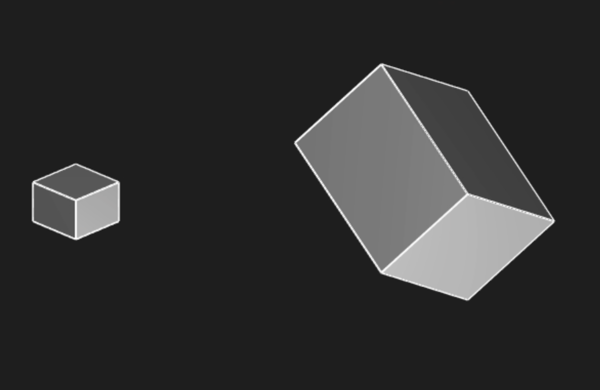
Default export
Here's a little time-saving feature for KCL exports. The last expression or variable declared in a KCL module is its default export. This means we could shorten our program
export fn cube(sideLength) {
  // Code omitted for brevity.
  // Same as previous example.
}

// This is the last expression in the module, so it's the _default export_.
cube(sideLength = 20)
and use it in main.kcl like this:
// main.kcl
import cube from "cube.kcl"
// Let's use the default export, and give it a name.
import "cube.kcl" as mySpecificCube

mySpecificCube |> translate(x = 50) |> rotate(pitch = 45)
secondCube = cube(sideLength = 7)
For more details, you can read the modules reference in the KCL docs.
Interop with other CAD programs
KCL tries to work well with the rest of the CAD ecosystem. That means you can use other CAD files and import them into KCL, or export your KCL to other formats for use with other CAD software. You can use the Zoo API or CLI to drive these conversions. Let's see how.
Importing other files into KCL
The import statement lets you load models from other CAD files and use them in your KCL. Once imported, they can be translated, rotated, cloned etc. For example, let's import a shape from some CAD file. If you place a file named "car motor.step" in the root of your KCL project (i.e. next to main.kcl), you can run this:
import "car motor.step" as motor
Once you've imported the geometry, it'll be placed in your scene. You can then modify it like any other KCL solid. For example, let's make two motors:
import "car motor.step" as motor

motor
  |> translate(x=10)
clone(motor)
  |> translate(x=20)
Exporting KCL into other formats
If you're writing KCL in the Zoo Design Studio, you can export your design into many different formats. Bring up the export menu via the Command Palette: just type Cmd+K on MacOS, or Ctrl+K on Windows/Linux. Type Export and press enter to choose the Export command. Then you can choose a format, and download your model! From there, you could import it into another CAD program, or send to a 3D printer or manufacturing service.
You can also use the Zoo CLI: just run
zoo kcl export --output-format gltf main.kcl model
Wrote file: model/output.gltf
Currently Zoo supports exporting and importing fbx, glb, gltf, obj, ply, step, and stl files.
Sketching 2D shapes
WARNING: This chapter covers the old syntax for our previous sketch library (that didn't support constraint solvers). If you're new to KCL, you should probably skip this chapter and read the new chapter on sketch blocks. If you've already got old KCL code that used the old syntax for sketching, don't worry, you can keep using the old syntax, and this chapter will explain it. But new users shouldn't worry about this, unless they're working with old code.
Let's use KCL to sketch some basic 2D shapes. Sketching is a core workflow for mechanical engineers, designers, and hobbyists. The basic steps of sketching are:
- Choose a plane to sketch on
- Start sketching at a certain point
- Draw a line from the current point to somewhere
- Add new lines, joining on from the previous lines
- Eventually, one line loops back to the starting point.
- Close the sketch, creating a 2D shape.
You can do each of these steps in KCL. Let's see how!
Your first triangle
Let's sketch a really simple triangle. We'll sketch a right-angled triangle, with side lengths 3 and 4.
Just copy this code into the KCL editor:
startSketchOn(XY)
  |> startProfile(at = [0, 0])
  |> line(end = [3, 0])
  |> line(end = [0, 4])
  |> line(endAbsolute = [0, 0])
  |> close()
Your screen should look something like this:
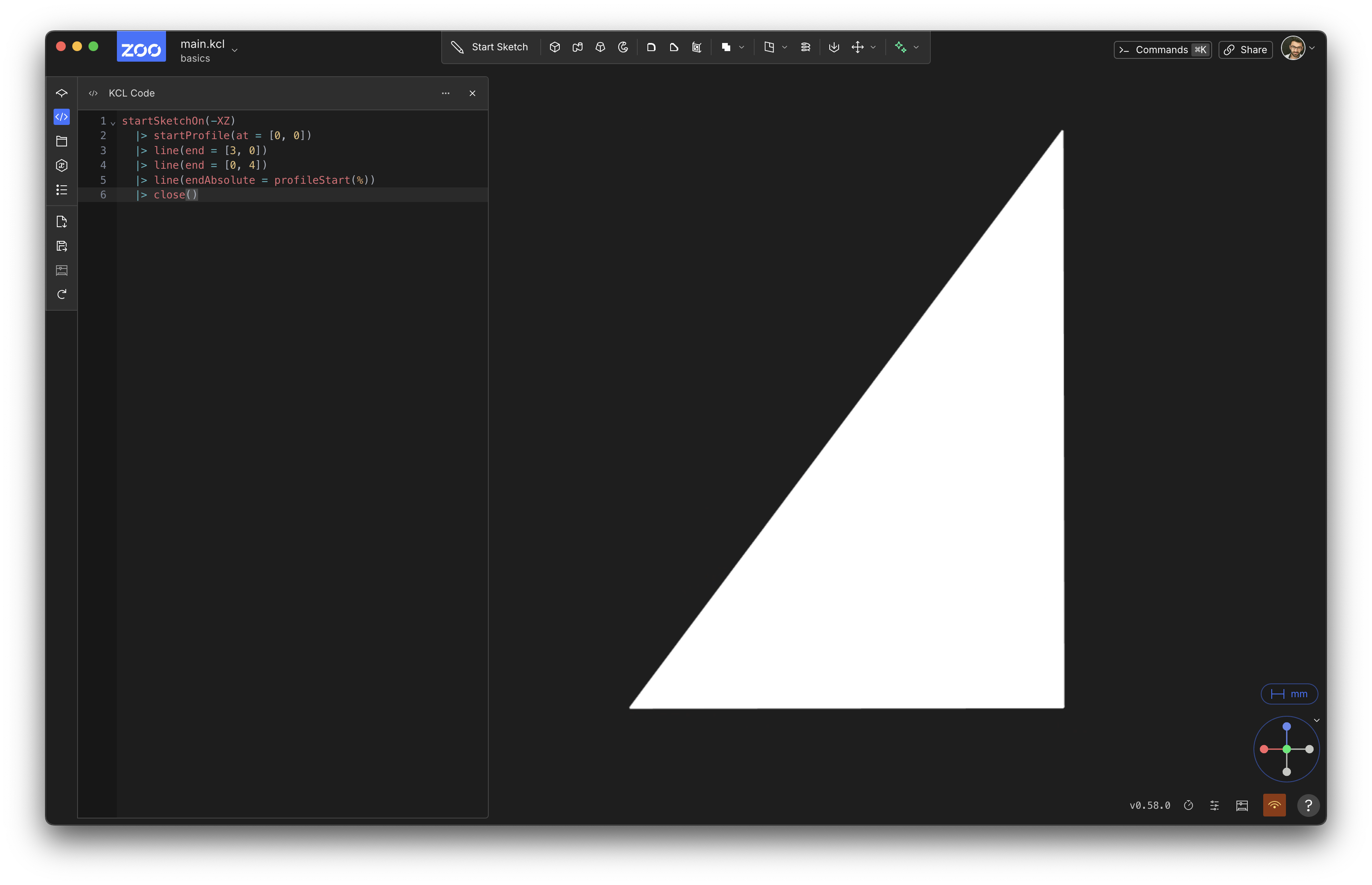
Congratulations, you've sketched your first triangle! Rendering your first triangle is a big deal in graphics programming, and sketching your first triangle is a big deal in KCL.
Let's break this code down line-by-line and see how it corresponds to each step of sketching from above. Note that each step in creating this triangle uses the pipeline syntax |>. This means every function call is being piped into the next function call.
1: Choose a plane
In KCL, there's six basic built-in planes you can use: XY, YZ, XZ, and negative versions of each (-XY, -YZ and -XZ). You can use one of these standard planes, or define your own (we'll get to that later). Those six standard planes can be used just like normal variables you define, except they're pre-defined by KCL in its standard library. You can pass them into functions, like the startSketchOn function. So, line 1, startSketchOn(XY) is where you choose a plane, and start sketching on it.
startSketchOn takes one argument, the plane to sketch on. It's the special unlabeled first parameter. We'll go over some other planes you can sketch on in the chapter about sketch on face.
2: Start sketching
Sketches contain profiles -- basically, a sequence of lines, laid out top-to-tail (i.e. one line starts where the previous line ends). We have to start the profile somewhere, so we use startProfile(at = [0, 0]). The startProfile takes two parameters:
- The sketch we're adding a profile with. This is one of those special unlabeled first parameters, so we don't need a label. We're setting it to the sketch from
startSketchOn(XY), which is being piped in via the|>. If you don't set this first parameter, it defaults to%, i.e. the previous pipeline expression. And that's exactly what we want! So we're leaving it unset. - The
atparameter indicates where the profile starts. For this example, we'll start at the origin of the XY plane, i.e. the point[0, 0].
3: Add paths
A profile is a sequence of paths. A path is some sort of curve between two points, possibly straight lines, circular arcs, parabolae, or something else. For this triangle, we're adding 3 paths, which are all straight lines. The line call says to draw a line starting at the previous end point. Currently, this is [0, 0] from the startProfile call. So this line starts at [0, 0]. Where does it end? Well, the line call says that end = [3, 0], which means "extend this line 3 units along the X axis, and 0 units along the Y axis". This is a relative distance, because it's telling you how far to move from the previous point. So, this line goes from [0, 0] to [3, 0].
4: Add more lines, joining on from previous lines.
The next call is line(end = [0, 4]). It draws a line from the previous line's end ([3, 0]), extending a distance of 0 along X and 4 along Y. So it goes from [3, 0] to [3, 4].
5: Join back to the start
Our third line heads back to the start of the profile, i.e. [0, 0]. We do this by calling line(endAbsolute = [0, 0]). Note that this uses endAbsolute =, not end = like the previous lines. The end = arguments were relative distances: they said how far away the new point is, along both X and Y axes, from the previous point. This one is different: this is an absolute point, not a relative distance. The array [0, 0] isn't saying to move 0 along X and 0 along Y. It's saying, draw a line that ends at the specific point [0, 0], i.e. the origin of the plane.
Because this is the same point that our profile starts at, this line has looped our profile back to its start.
We could have also used a relative line here, and looped back to the start with line(end = [-3, -4]). That would achieve the same thing. But this requires manual calculation. You, the programmer, have to look at all the previous lines and figure out how where the last line starts, and then "undo" all that distance by putting a line with the negative X and Y distances (so that the line goes back to the origin). In our example, this was easy, but in real-world designs this might be very tough! And even when it's easy, using an absolute point here communicates our intent better. We're just want to draw a line that returns to the start point. We don't really care about the distance here.
It doesn't really matter which one you use, although note that Zoo Design Studio will usually prefer relative lines for almost everything. Closing a sketch is the one exception where Zoo Design Studio will use an absolute line.
Now, if we stopped our program here, you could see all three lines:
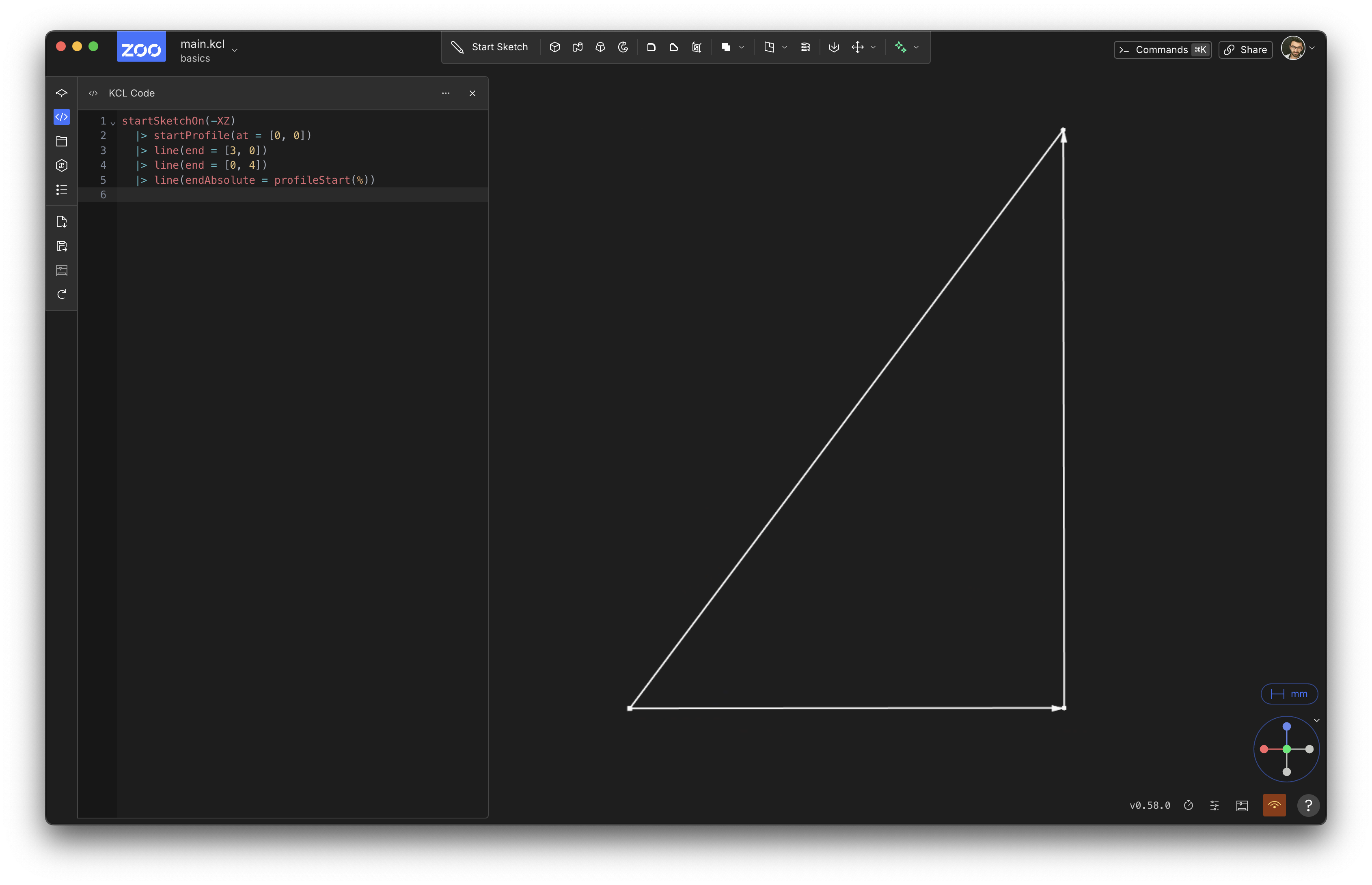
Note that the relative lines (i.e. the first two line calls, with end =) have arrows showing where they're going. This last line, which ends at an absolute point, does not.
6: Close the sketch
The last function being called is close. It takes one argument, the sketch to close. As in the previous functions, it's an unlabeled first parameter, so you could write close(%), but close() will do the exact same thing.
Once we add the close() call, the rendering changes from just 3 lines (like in the second image in this page) to a filled-in shape (like in the first image on this page).
Enhancements
This code totally achieved our goal: it sketches a right-angled triangle with sides of length 3 and 4. Mission accomplished.
Of course, in programming, there's usually several different ways to achieve a goal. KCL is no different! Let's look at some different ways we could have sketched this shape.
Closing shapes
One important principle in programming is "don't repeat yourself" (DRY). Look back at this code: it uses the point [0, 0] twice. Once when we start the sketch, and once when we close the sketch. There's nothing necessarily wrong with this, but if you want to change the triangle later, you'll have to change this in two different places. And if you make a typo in one of the places, the model will break, because the sketch will be starting and finishing at a different point. This program doesn't have a bug currently, but by repeating this value twice, we introduce a potential bug in the future. I'd call this program brittle -- it's not broken, but it could break in the future. If we could define the point [0, 0] just once, the program would be more resilient, i.e. less likely to break if you change something in the future.
Here's a few ways to make this code less repetitive, less brittle, and DRY-er.
Firstly, you could replace [0, 0] with a variable like start, and use it in both places.
start = [0, 0]
startSketchOn(XY)
  |> startProfile(at = start)
  |> line(end = [3, 0])
  |> line(end = [0, 4])
  |> line(endAbsolute = start)
  |> close()
Next, we could use a helper function profileStart instead.
startSketchOn(XY)
  |> startProfile(at = [0, 0])
  |> line(end = [3, 0])
  |> line(end = [0, 4])
  |> line(endAbsolute = profileStart())
  |> close()
The profileStart function takes in the current profile, and returns its start value. It takes a single unlabeled parameter, which we're setting to % (the left-hand side of the |>). Like always, if the special unlabeled argument is set to %, you can just omit the %, because that's the default.
X and Y lines
The first line of our triangle is parallel to the X axis, and the second line is parallel to the Y axis. This means we could simplify our code somewhat by using the xLine and yLine functions:
startSketchOn(XY)
  |> startProfile(at = [0, 0])
  |> xLine(length = 3)
  |> yLine(length = 4)
  |> line(endAbsolute = profileStart())
  |> close()
xLine takes an unlabeled first parameter for the sketch (which, as before, we're setting to % and can therefore omit) and then a length parameter, which tells KCL to draw a flat line, parallel to the X axis, with the given length. Basically,xLine(length = n) is a neater way to write a horizontal line like line(end = [n, 0]). You can use whichever one you prefer. The yLine function works the same way, but for vertical lines.
These examples use relative xLine and yLine -- i.e. lines that end a certain distance away from the previous point. If you want to instead draw a line to a specific point along the X axis (like x = 3), you could use xLine(endAbsolute = 3).
Conclusion
We've written our first triangle. We learned:
- Sketches are on some plane, and KCL includes standard planes XY, YZ and XZ (and their negative versions, which point the third axis in the opposite direction).
- Sketches contain profiles, which are made of sequential paths. In our example, there's one profile, a triangle, made of three paths (3 straight lines).
- Lines start at the end of the previous point (the first line starts at the
startProfile(at=)point) - Lines can end either a certain distance away along X and Y (a relative end), or at a particular point along the plane (an absolute end)
- The
closefunction turns a sequence of paths that form a loop into a single 2D shape.
Sketching curved lines
WARNING: This chapter covers the old syntax for our previous sketch library (that didn't support constraint solvers). If you're new to KCL, you should probably skip this chapter and read the new chapter on sketch blocks. If you've already got old KCL code that used the old syntax for sketching, don't worry, you can keep using the old syntax, and this chapter will explain it. But new users shouldn't worry about this, unless they're working with old code.
In the previous chapter, we sketched a basic triangle. In this chapter, we'll look at some more interesting kinds of sketches you can do, using more interesting kinds of paths.
Pills
Let's sketch a pill shape, like a rectangle but with rounded edges. We can use tangential arcs for this. The tangentialArc function sketch a curved line -- specifically, an arc, or a subset of a circle -- starting from the previous line's end. It draws it at a smooth angle from the previous line, i.e. tangent to the previous line.
height = 4
width = 8
startSketchOn(XZ)
  |> startProfile(at = [0, 0])
  |> xLine(length = width)
  |> tangentialArc(end = [0, height])
  |> xLine(length = -width)
  |> tangentialArc(endAbsolute = profileStart())
It should look like this:
Let's analyze this! It looks very similar to the triangle we sketched previously, but we're using tangentialArc. You can see it takes a relative end, i.e. an X distance and Y distance to move from the current point. It draws a nice smooth arc there.
We wrote this arc using end, i.e. an X and Y distance. But we could have defined this arc differently, using a radius and angle instead (or a diameter and angle). You can replace the tangentialArc(end = [0, height]) with tangentialArc(angle = 180, radius = height) instead, and it should draw the same thing.
height = 4
width = 8
startSketchOn(XZ)
  |> startProfile(at = [0, 0])
  |> xLine(length = width)
  |> tangentialArc(diameter = height, angle = 180deg)
  |> xLine(length = -width)
  |> tangentialArc(endAbsolute = profileStart())
Here, the angle 180deg is measuring a counterclockwise angle. To make the arc go the other direction (clockwise), you'd use -180deg.
The second tangentialArc call takes an absolute point. We tell it to draw an arc from the current point to the start of the profile. This should remind you of how straight lines can use either end (relative) or endAbsolute.
Spirals
We can use tangential arcs to make a spiral too.
height = 100
startSketchOn(XZ)
  |> startProfile(at = [0, 0])
  |> tangentialArc(angle = 180, radius = height)
  |> tangentialArc(angle = 180, radius = height * 1.1)
  |> tangentialArc(angle = 180, radius = height * 1.2)
  |> tangentialArc(angle = 180, radius = height * 1.3)
  |> tangentialArc(angle = 180, radius = height * 1.4)
  |> tangentialArc(angle = 180, radius = height * 1.5)
  |> tangentialArc(angle = 180, radius = height * 1.6)
  |> tangentialArc(angle = 180, radius = height * 1.7)
It should look like this:
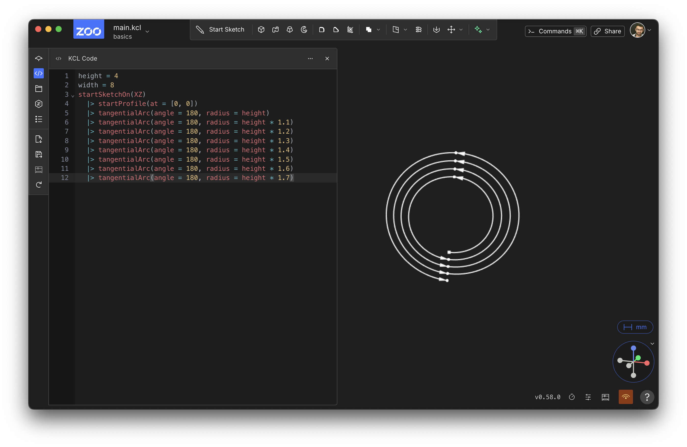
This works because each tangentialArc is drawing half a circle, away from the previous arc, and the circle is getting slightly larger each time. The 180 is a counterclockwise angle, so each time we draw a new arc, it bends around the circle counterclockwise.
Circles
And lastly, let's look at the humble circle.
startSketchOn(XZ)
  |> circle(center = [0, 0], radius = 10)
The circle call takes center and radius arguments. Note that circle closes itself without any need for a close() call. That's because a circle is inherently closed -- it always starts and ends its own profile.
Reduce and geometry
WARNING: This chapter covers the old syntax for our previous sketch library (that didn't support constraint solvers). If you're new to KCL, you should probably skip this chapter and read the new chapter on sketch blocks. If you've already got old KCL code that used the old syntax for sketching, don't worry, you can keep using the old syntax, and this chapter will explain it. But new users shouldn't worry about this, unless they're working with old code.
- Sketching a square with reduce
- Sketching a parametric polygon with reduce
- Repeating geometry with reduce
The reduce function lets us iterate over an array, consuming its contents and reducing them down to one single item. Reduce is a very powerful, flexible tool. It can be complex too, but that complexity lets us do some very interesting things.
For example: how would you write a KCL function that produces an n-sided polygon? This is an ambitious project, so let's start with something simpler, and build back up to an n-sided polygon.
Sketching a square with reduce
Can we use reduce to make a square function, first? Once we've done that, we can make a parametric sketchPolygon function that works like square when the number of sides is 4, but can just as easily produce hexagons, octagons, triangles, etc.
fn square(sideLength) {
  emptySketch = startSketchOn(XY)
    |> startProfile(at = [0, 0])
  angle = 90
  fn addOneSide(@i, accum) {
    return angledLine(accum, angle = i * angle, length = sideLength)
  }
  return reduce([1..4], initial = emptySketch, f = addOneSide)
    |> close()
}

square(sideLength = 10) |> extrude(length = 1)
What's going on here? Let's break it down. We declare fn square which takes one argument, the sideLength. We create an initial empty sketch (at [0, 0] on the XY plane), and declare that the angle is 90.
Next, we declare a fn addOneSide. It takes in two arguments: i, which represents the index of which side we're currently adding, and accum, which is the sketch we're adding it to. This function adds one angled line to the sketch. The line's side is whatever side length was given, and its angle is 90 times i. So, the first line will have an angle of 90, the second 180, the third 270, and the last 360.
Then we call reduce, passing in the array [1, 2, 3, 4], setting the initial accumulator value to the empty sketch we started above, and calling addOneSide every time the reduce handles an array item. When reduce runs, it:
- Starts
accumas the empty sketch - Handles the first item,
i = 1, callsaddOneSide, which takes the previous accumulated sketch (currently empty) and adds an angled line at 90 degrees. This becomes the next accumulated sketch. - Handles the second item,
i = 2, callsaddOneSide, which takes the previous accumulated sketch (with a single line) and adds an angled line at 180 degrees. This becomes the next accumulated sketch. - For
i = 3, it takes the accumulated sketch with two lines, and adds a third line, similar to the previous step. - For
i = 4, it takes the accumulated sketch with three lines, and adds a fourth line, similar to the previous step.
Thus it builds up a square.
Sketching a parametric polygon with reduce
OK! We've seen how to use reduce to add lines to an empty sketch. We're ready to make our polygon function. Although, KCL already has a polygon function in the standard library. So, to avoid clashing with the existing name, we'll call ours sketchPolygon.
We can start with our square function and generalize it. First, we'll add an argument for the number of lines.
fn sketchPolygon(@numLines, sideLength) {
}
We can use the same initial empty sketch. We'll have to change angle, because it won't be 90 anymore. The angle now depends on how many edges the shape has:
angle = 360 / numLines
And lastly, our reduce call will need to take an array of numbers from 1 to numLines, not 1 to 4. So we'll use [1..numLines] as the first argument to reduce.
Let's put all that together:
fn sketchPolygon(@numLines, sideLength) {
  initial = startSketchOn(XY)
    |> startProfile(at = [0, 0])
  angle = 360 / numLines
  fn addOneSide(@i, accum) {
    return angledLine(accum, angle = i * angle, length = sideLength)
  }
  finished = reduce([1..numLines], initial = initial, f = addOneSide)
  return finished |> close()
}

sketchPolygon(7, sideLength = 10) |> extrude(length = 1)
pattern2D and pattern3D, so we hope to add a pattern1D eventually, so that these complicated reduces won't be necessary. Until then, reduce can be a good way to implement tricky functions like sketchPolygon.
Repeating geometry with reduce
Let's look at another way to use reduce. Say you're modeling a comb, with a parametric number of teeth. We can use reduce to solve this again:
fn comb(teeth, sideLength) {
  toothAngle = 80
  handleHeight = 4
  initial = startSketchOn(XY)
    |> startProfile(at = [0, 0])

  // Sketches a single comb tooth
  fn addTooth(@i, accum) {
    // Line going up
    return angledLine(accum, angle = toothAngle, length = sideLength)
      // Line going down
      |> angledLine(angle = -toothAngle, length = sideLength)
  }
  allTeeth = reduce([1..teeth], initial = initial, f = addTooth)
  finalComb = allTeeth
    // Add the handle: a line down, across, and back up to the start.
    |> yLine(length = -handleHeight)
    |> xLine(endAbsolute = 0)
    |> yLine(endAbsolute = 0)
    |> close()
  return finalComb
}

comb(teeth = 10, sideLength = 10) |> extrude(length = 1)
We write a function addTooth which adds a tooth (going up, then back down) to a sketch. Using reduce, we can call that function teeth times. Each time, the new tooth gets appended to the end of the sketch path. Once we've drawn all the teeth, we draw a simple handle leading back to the start.
reduce is a powerful way to make parametric designs, repeating geometric features as many times as you need. You can design parametric polygons with a variable number of sides, or repeat geometry linearly (like we did for our comb).