Zoo CAD Engine Overview
- 1 Introduction
- 1.1 Motivation: Why Build a CAD Engine?
- 1.2 A Comparison Between CAD and Game Engines
- 1.3 CAD Software Performance
- 2 Core Design Principles and Methodology
- 2.1 CAD-as-a-Service
- 2.2 Modelling Paradigms
- 3 Implementation of Key Features
- 3.1 Sweeps
- 3.2 Patterns and Duplication
- 4 Case Study: GPU-Accelerated Surface-Surface Intersection (SSI)
- 4.1 Introduction to SSI
- 4.2 Background: NURBS and Standard SSI Approaches
- 4.2.1 Why NURBS?
- Applications of SSI in NURBS
- 4.2.2 Standard SSI Approaches for NURBS
- 4.3 The Zoo GPU-Friendly SSI Methodology
- 4.3.1 Rationale for GPU Acceleration
- 4.3.2 Patented Algorithm Overview
- 4.3.3 Parameter Space Processing
- Branching
- 4.3.4 Curve Reconstruction and Refinement
- 5 References
1 Introduction
A CAD engine (often called a CAD kernel) is responsible for representing the model geometry such as B-Rep, NURBS, CSG etc., and for executing the common operations performed by CAD software such as extrusion, revolution, lofting, etc. CAD engines come in many different flavors, depending mostly on the application domain.
SketchUp, for example, grew out of the architectural design community who appreciated the easy-to-learn, intuitive interface. Architects could quickly ‘sketch up’ an idea and access a variety of rendering modes suited to their needs. In order to achieve such a flexible and easily understandable user interface, SketchUp relied on polygons as geometric primitives. Precision, complex surfacing, full solid modeling (knowing inside from outside) were not supported initially. Most building designs did not require such tools. Even boolean operations of union, intersection and difference had minimal (polygonal) support and lacked robustness.
In contrast, Siemens NX had roots in aerospace (McDonnell Douglas). Sophisticated curved surfaces geometries like airfoils or turbine blades were fundamental and were often the start point for design. Precision could mean the difference between success or failure. Robust solid modeling underpinned critical mass properties and physics simulations. The user interface was, as a result, much deeper and more intricate, often requiring years to fully master. (The user license was, as a consequence, far more expensive).
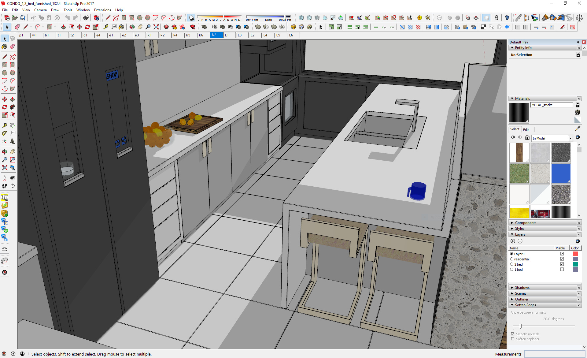
Figure 1: SketchUp. A user-friendly, conceptual tool with polygon-based modeling.
Credit: SketchUp Forums
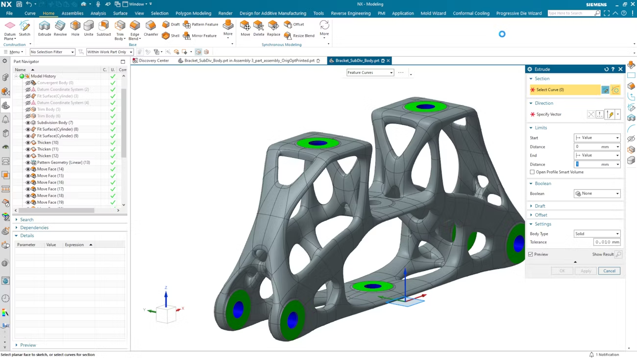
Figure 2: Siemens NX. A precision engineering tool with NURBS-based modeling.
Credit: Siemens Digital Industries Software
Over the years both modelers have migrated towards each other; SketchUp has added limited surfaces and some aspects of solid modeling, while Siemens have improved UI and visualization tools. There is only so much that can be done, however, with fundamentally different mathematical algorithms and code bases. Also the expectations of the user communities vary wildly, driven by years of training and use.
We have highlighted only two modelers; the entire landscape of modeling is huge, diverse, and application focussed.
1.1 Motivation: Why Build a CAD Engine?
Traditionally, so many people look up at a mountain and say "that's too tall, and it has already been climbed, so why bother?" It is difficult to gain additional insight about how to solve existing problems differently if one lacks the perspective from the journey to and from the top of that mountain. Perhaps the established route of ascent is crumbling. Is there a more efficient way to the top that has only recently been discovered? Are there new technologies that have been recently invented to aid in the climb?
Shying away from difficult problems often leads us to be stuck with the same situations without learning from our past. Remaining flexible about where bottlenecks or other problems lie is equally important. We are pretty determined to solve these problems with traditional CAD engines. Currently, we are opting to solve as many problems as we possibly can with our own CAD engine. This provides us the benefits of perspective on CAD engine design, alongside the flexibility to solve problems for our customers with surgical precision that the rest of the industry lacks.
1.2 A Comparison Between CAD and Game Engines
What could a CAD engine possibly have to do with a game engine? As the late 90’s came to a close, hardware accelerator cards, driven by chips today better known as GPUs, began to become widely available to PC consumers. These magical little devices allowed PC software to render far more 3D polygons than previously possible at interactive speeds. This paradigm shift in technology occurred well over a decade after most of the CAD kernel software that we still use today has been written. A few years later, graphics hardware manufacturers began allowing general purpose programming on GPUs (GPGPU). It turns out, many of the geometric operations needed by CAD algorithms lend themselves naturally to the massively parallel nature of GPU computing. Furthermore, it turns out that the techniques needed to render the CAD display are identical to the techniques used by 3D video game engines to render the game world. Additionally, the low-level mechanics of managing compute shaders to do complex work on the GPU are fundamentally the same between CAD software, 3D modeling software, and game engine software. While over the last several decades, gaming has pushed the state of the art in 3D graphics rendering alongside GPU computing, CAD software has not.
Most existing CAD programs today allow you to quickly create more content than they can efficiently render in a few steps. Ask any engineer who has driven their CAD program too hard, and they’ll share their stories of frustration. At Zoo, we believe the GPU has been under-leveraged on both sides of the CAD engine pipeline: The geometry engine and the rendering engine. If either of these systems are bottlenecked, the user experience is going to suffer. Our research is centered around employing modern techniques from all fields of computer science, to design a more performant CAD engine.
1.3 CAD Software Performance
Ever wondered specifically what makes CAD software slow? This is a complicated question, but it generally boils down to a combination of software bloat, resource constraints, and legacy. A 3D authoring tool is only as fast as the sum of its components. If any of those components are slow, then the software is slow. Generally, modern CAD software is a combination of legacy CAD kernels wrapped by programming languages and frameworks that are liberal with compute resource usage. For example, if every 3D edge in your model requires the creation of a C# object to store its ID, then the software is now using up more significantly memory than is required to efficiently store that information.
This type of systemic bloat often results in simple CAD operations using far more computational resources than are strictly required to perform the task at hand. Running all of this software on anything but the highest performance computer hardware can be a recipe for performance problems that significantly degrade the user experience.
Another factor contributing to CAD software performance challenges is the 'combinatorial curse' introduced by the number of different geometric primitives that many systems support. As CAD systems evolve, they often accumulate different representation formats (polygons, NURBS, subdivision surfaces, etc.) to accommodate various use cases. This proliferation of primitives means that every operation must have multiple implementations: polygon-to-polygon, polygon-to-NURBS, NURBS-to-NURBS, and so on. The number of operational combinations grows factorially with each new primitive type added to the system. A performance bottleneck then emerges when traversing the B-Rep database, as the software must first determine which primitives are involved before selecting the appropriate operation implementation. Modern CAD software often spends more time walking these data structures than performing actual geometric computations. This approach is also inherently unfriendly to GPU acceleration, which thrives on uniform operations across consistent data structures.
We aim to address this problem by maintaining a minimal set of geometric primitives. Rather than implementing specialized representations for features like fillets, we represent these as B-splines with specific constraints. This way, operations only need to handle B-splines, allowing us to develop highly optimized, GPU-friendly algorithms like our surface-surface intersection method. By avoiding the combinatorial explosion of primitive interactions, we can achieve significant performance improvements over existing CAD systems.
2 Core Design Principles and Methodology
2.1 CAD-as-a-Service
Most CAD-as-a-Service systems are built around the idea of retrofitting legacy CAD systems to be consumable from an API across the web. While this idea certainly can work, we have the added benefit of designing our CAD engine to be directly interoperable with our CAD API. This affords us opportunities for optimization such as batch processing, parallelization of independent CAD workflows, pre-emptive resource allocations, and more.
Beyond these affordances, when you retrofit an API onto existing software, you often only expose a subset of your possible software via the API. There is often extra functionality that the first-party application can use, which can’t be accessed by the API. This means the first-party app has inherent advantages over third-party integrations. By designing Zoo from the ground up to always use an API, we ensure that third-party developers always have access to the exact same functionality that our employees do. There's no secret fast mode available to the Zoo team but not to external developers. When you build on our API, you're using the exact same tools we use to build our app.
2.2 Modelling Paradigms
B-Reps are a standard starting ground for CAD representations. They offer parametric, concise descriptions of surfaces that can be easily recreated by engineers who understand basic geometry. Implicit/SDF-based solutions like those driven by dual-contouring algorithms are extremely impressive, but do have their own drawbacks for simple (common CAD workflow) shapes and surfaces. To extract a perfect B-Rep representation from an implicit surface, the software essentially must work its way backwards from a densely tesselated structure of faceted faces through complex topology optimization. This is a costly operation that can result in inaccuracies with needlessly complex results.
Additionally, Implicit modeling usually requires a large 3D compute space. This is usually in the form of a 3D grid or spatial tree data structure in which the amount of sheer compute work grows polynomially () with the size of the structure you're working on. While various compute-space optimizations help mitigate this problem, ultimately SDF has a scaling problem that runs up against the limited resource of GPU memory needed to run these types of algorithms quickly.
3 Implementation of Key Features
3.1 Sweeps
Sweeping a shape about a general trajectory curve is a commonly performed CAD operation. It is no trivial task to implement general sweeps for CAD. However it can be helpful to break it down into individual steps as a window into how such a feature is implemented within the KittyCAD engine.
Generally speaking a Sweep is a general extrusion of a section curve about a general trajectory curve1.
Where:
- is the closed profile curve.
- is a general trajectory curve.
- is a general orientation function used to correctly orient the section as it sweeps across the trajectory. It is general, and could be valued as either a 3x3 orthonormal matrix or a quaternion.
To be usable in a CAD engine, must be computable in NURBS form1:
Where:
- .
As an example, consider constructing a semi-circular profile curve. This curve can be described programmatically as follows:
Which yields:
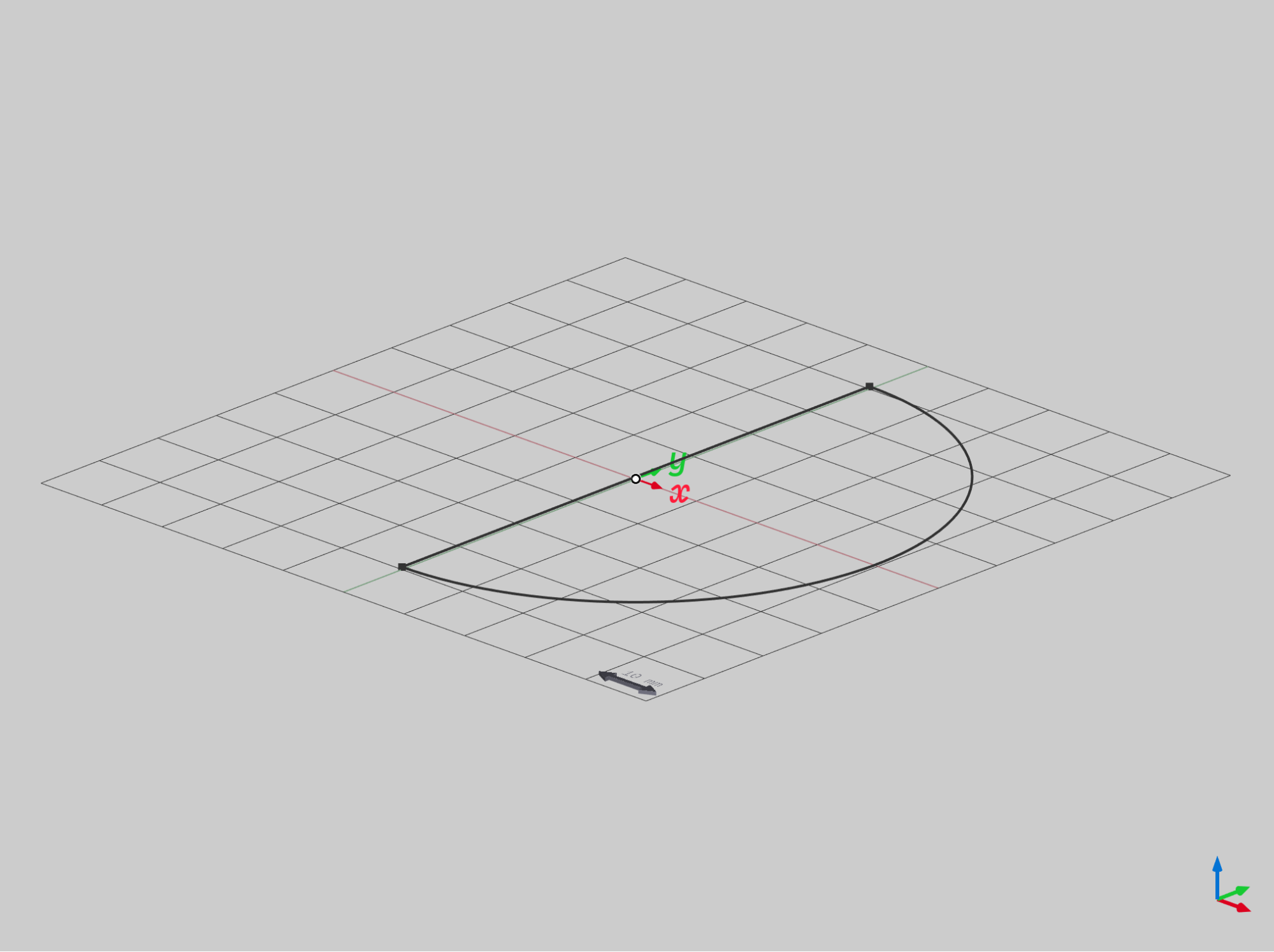
Figure 4 - A semi-circular profile curve, suitable as a sweep section.
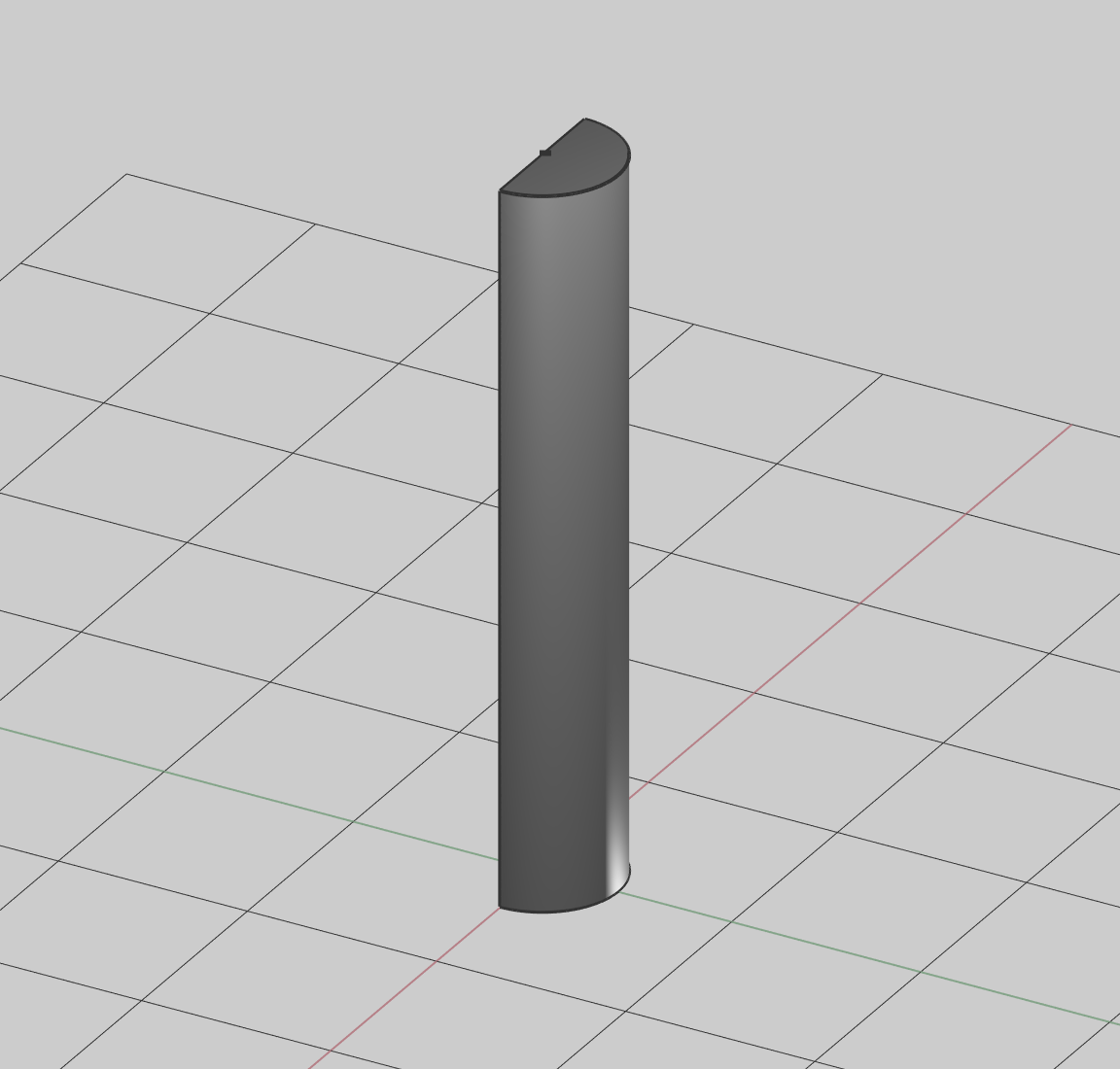
If is a perpendicular straight line, then simplifies to an extrusion surface with for all . Similarly, if is an arc, then will be the surface of revolution.
Figure 5 and Figure 6 illustrate the case where a sweep simplifies to an extrusion.
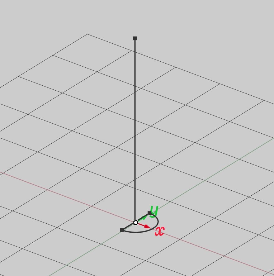
Figure 5: Sweep profile and perpendicular trajectory curve.
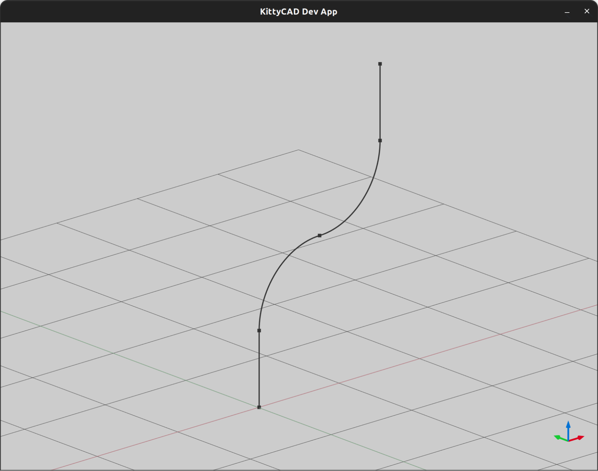
In the case where is curved and general, the swept surface can be constructed by a skinned interpolation of cross sections.
This can be described programmatically:
Figure 7 shows the trajectory curve, Figure 8 shows the transformed (re-oriented) section instances, and Figure 9 shows the resulting solid that is yielded by performing a loft operation on the transformed sections.
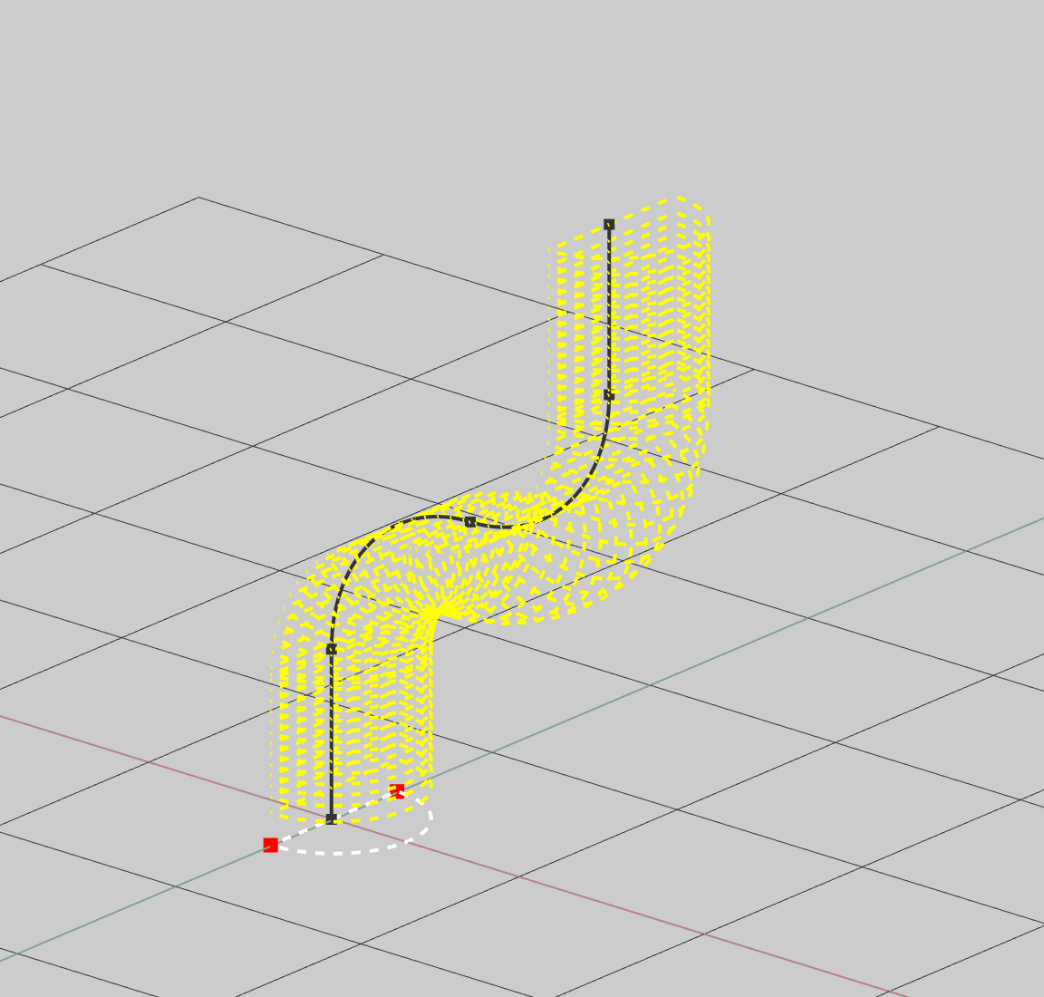
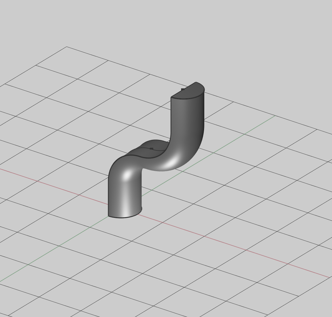
The astute reader might notice that the trajectory curve from figure 7 can be decomposed into a series of straight lines and arcs. Thus, in cases where higher-order surface continuity is not globally required, this sweep can be re-expressed as a combination of extrusion and revolutions with much less computational work.
It is worth noting that individual swept surfaces must be combined topologically to form a valid B-Rep that is usable for CAD applications. This is an important step in the sweeping algorithm as it reduces the global complexity of any individual B-Rep face. Essentially, each discrete path component of the decomposed section curve source is individually swept by each individual discrete path component of the decomposed trajectory curve . This produces separate surfaces where is the number of path components of the section curve (2 in our example) and is the number of path components in the trajectory (4 in our example). These faces are trivially converted to untrimmed square B-Rep faces with edges that lie on the boundaries of their respective evaluated surfaces. For open trajectory curves, two additional end-cap faces are added which correspond to the oriented section instances at the very beginning and very end of the sweep trajectory. Finally, all of these separate faces are combined to a solid manifold B-Rep via a join algorithm which merges all faces with coincident edges.
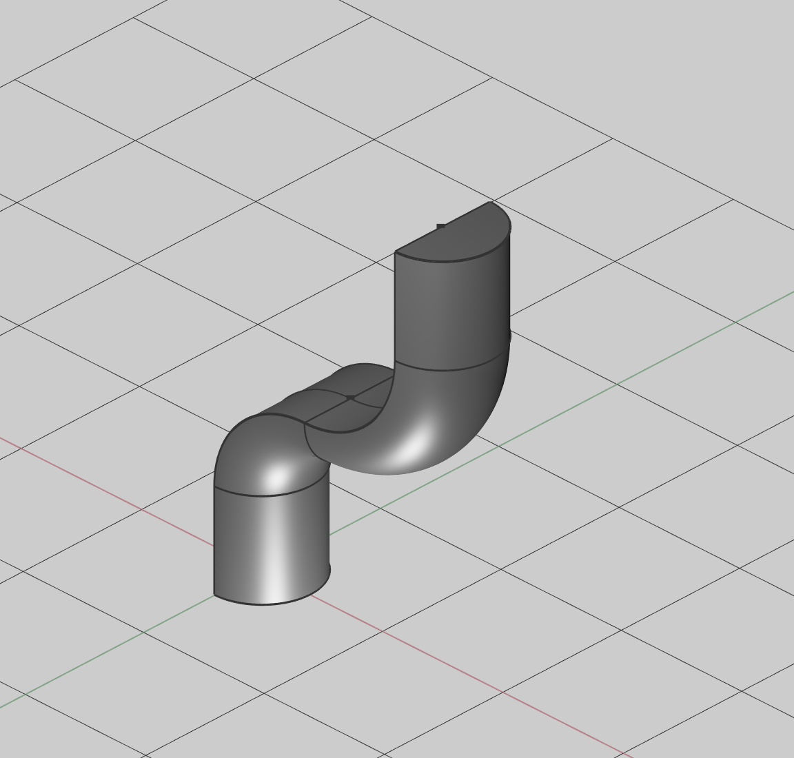
Figure 10 - The swept solid B-Rep formed as a combination of extrudes and revolves as a join of 10 separate faces
Another issue with sweeps along the trajectory is that of managing the curvature of the trajectory curve. If the curve turns too abruptly it can undesirably cause the surface to self intersect, that is, to overlap with itself. This can be controlled by limiting the curve’s maximum curvature where the curvature is given by
Where is a vector-valued function defining a curve in 3D space, and is the parameterization of the curve:
For specific applications it is helpful to segment the trajectory curve such that each piece does not exceed the max curvature chosen on the max size of the sweep cross section. In this way intermediate interpolation stages are placed at segment endpoints which guarantees no foldovers of the sweep. The figure below shows a curve segmented into different colors by a given max curvature.
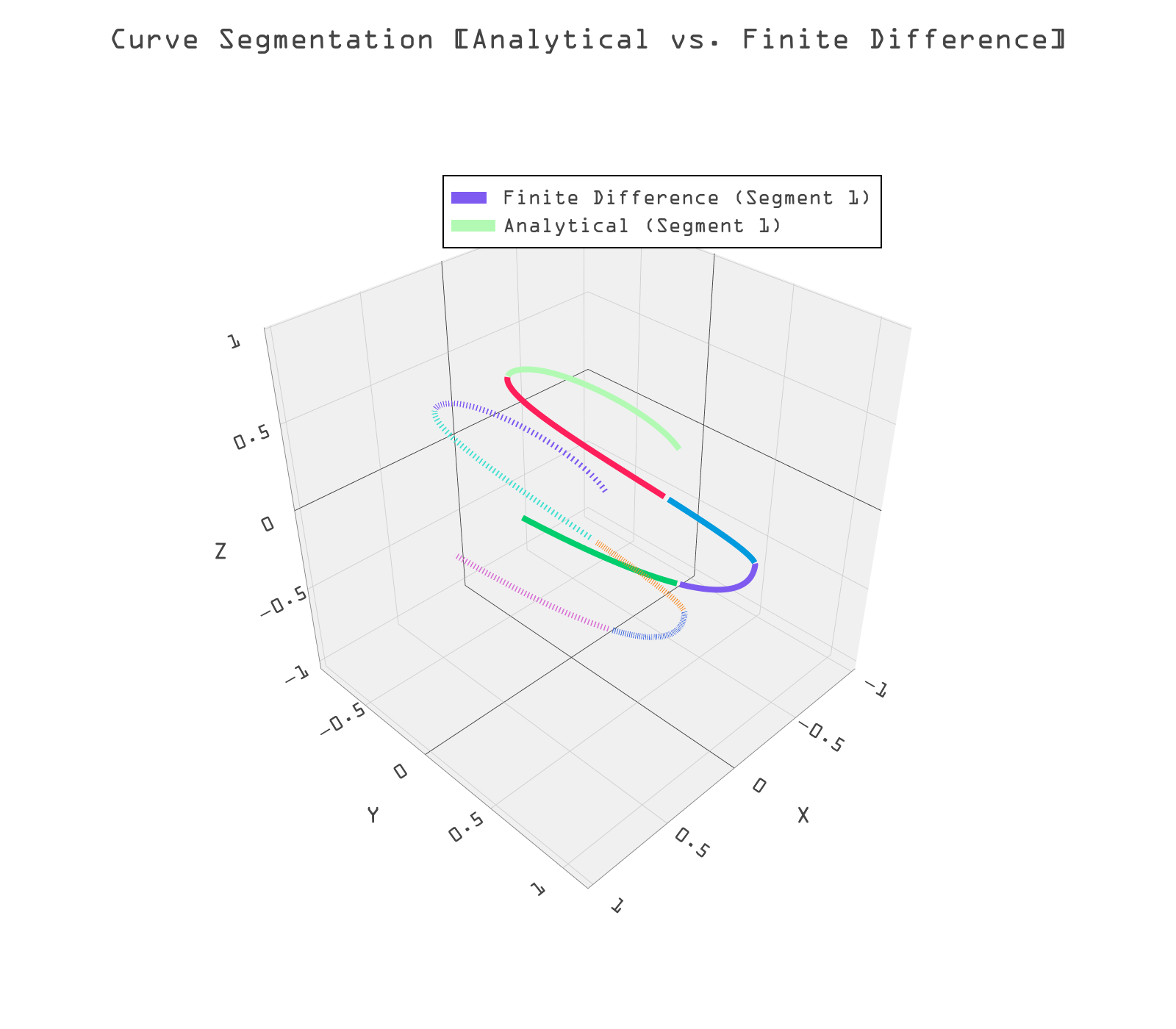
Figure 11: Segments computed both analytically and with finite differences. Analytical segments are solid, with finite difference dotted. This shows that the faster finite difference method is very close to the analytical one.
3.2 Patterns and Duplication
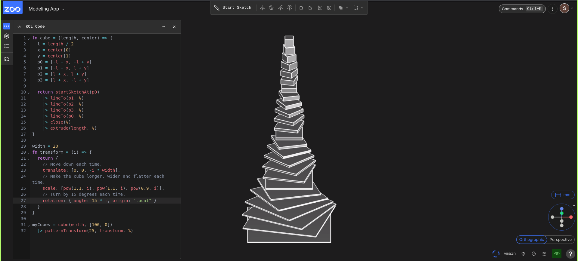
Figure 12: Examples of linear, circular, and array patterns.
It’s not unusual for a mechanical design engineer to want to place many duplicates of an object in a circle, array, line, or otherwise semi-uniform placement. Hand placement is tedious and often inaccurate, hence the need for a more automated way to duplicate geometry uniformly. Since its development, Zoo’s patterns have been highly used and many requests for ways to expand the usage of patterns have been made - they are just that powerful!
The underlying mathematics of patterns consists of transformation matrices that are produced using the user’s inputs. These operations aren’t super costly, with respect to runtime and memory, when performed on only a handful of objects. Most practical use cases can be rendered efficiently. Still, it’s not in the Zoo spirit to stop at what’s easy! The Zoo engine team has decided to move towards instancing patterned geometry, producing one render call to limit the time and memory resources used during the transfer from CPU to GPU. This means that the perceived runtime of patterning geometry stays fairly consistent, even with large adjustments to the number of duplicates rendered.
4 Case Study: GPU-Accelerated Surface-Surface Intersection (SSI)
4.1 Introduction to SSI
Surface-surface intersection (SSI) is a critical operation in CAD/CAM (Computer-Aided Design and Computer-Aided Manufacturing), which involves determining the curves where two or more surfaces meet. This process enables designers to create complex geometries, ensures the accuracy of manufacturing processes, and facilitates the analysis of assemblies in engineering applications. The challenge lies in the mathematical complexity of accurately computing intersections, especially for intricate shapes or when surfaces are defined by parametric equations. Miscalculations can lead to manufacturing defects or design flaws. Applications of surface-surface intersection are widespread, including in automotive design, aerospace engineering, architectural modeling, and product design, where precise fitting and assembly of parts are crucial.
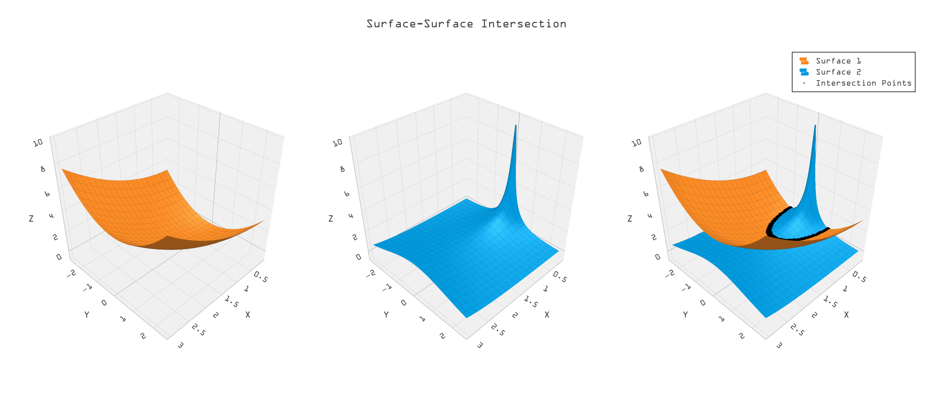
Figure 13: The meeting of two surfaces creates difficult-to-find intersection curves.
Precise geometric modeling is crucial for industries that require complex surface operations, such as aerospace, automotive, and consumer product design. The importance lies in several key areas:
- Validity.
- Imprecision, especially in SSI, can create fundamental differences between design intent and results Sometimes small inaccuracies result in major differences in topology and design.
- Part fit.
- Consistently precise models ensure that components fit together correctly over many version updates, reducing costly manufacturing defects or performance issues.
- Simulation and analysis.
- Accurate representations are necessary for usable simulations in fields like fluid dynamics, heat flow, collision detection, and stress analysis.
- Customization and flexibility.
- Industries often require specialized designs; precise modeling enables customization while maintaining general structural integrity and aesthetic appeal.
- Collaboration.
- In complex projects, teams need to coordinate and work simultaneously. Having a consistent and precise model ensures that everyone is aligned, reduces miscommunication and enhances collaboration across various disciplines.
Overall, consistent precision modeling underpins innovation and efficiency in industries where complex surface designs are found..
4.2 Background: NURBS and Standard SSI Approaches
4.2.1 Why NURBS?
Non-Uniform Rational B-Splines (NURBS) are a mathematical representation widely used in computer graphics, CAD, and modeling for representing curves and surfaces. They provide great flexibility and precision in creating complex shapes, NURBS are defined by control points, which enhance design flexibility, and enable them to represent both standard geometric shapes (like lines and circles) and free-form surfaces. Additionally, their ability to easily scale and modify makes them an industry standard in any domain requiring high-quality surface representation. Some popular software packages that utilize NURBS for design and modeling include Autodesk Alias, Rhino, Siemens NX, and CATIA.
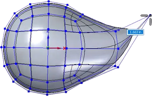
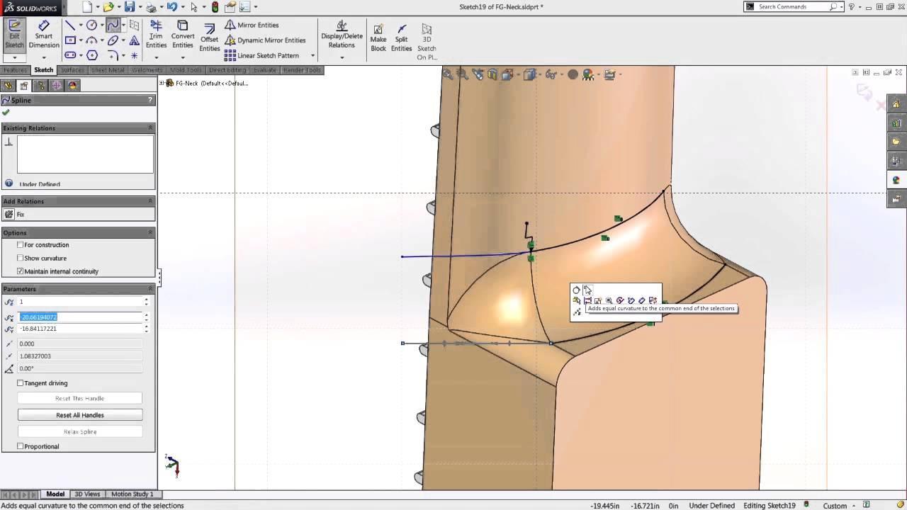
Figure 14: Easily manipulated mesh and control points (shown in blue) dictate the shape of a smooth object.
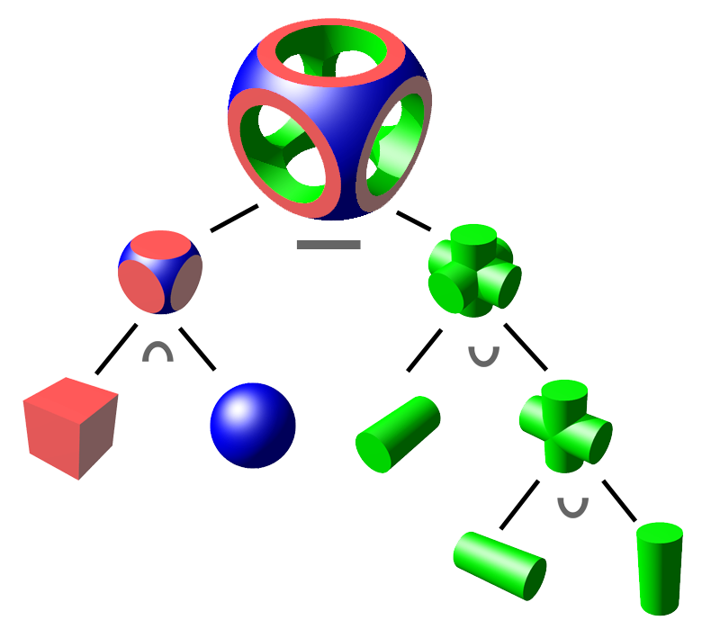
Applications of SSI in NURBS
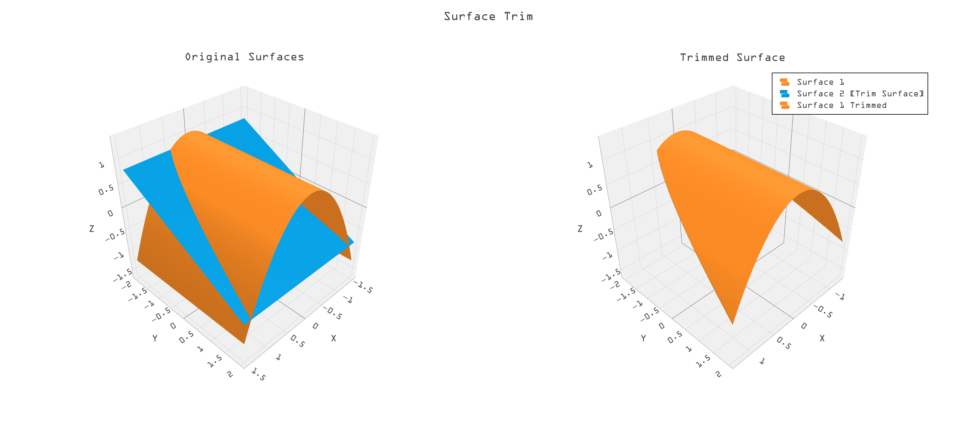
Boolean operations, trimming, blending, stenciling, and cut-away views for design and manufacturing all generate SSIs. These operations are illustrated in Figures 15 to 17.
4.2.2 Standard SSI Approaches for NURBS
Intersecting meshes is perhaps the easiest and fastest SSI method for NURBS. It consists of making a polygonal mesh out of both surfaces and then using the polygonal approximations to intersect. To intersect polygonal meshes, one can use various computational geometry techniques. One common method is to bound volume hierarchies (BVH) to quickly eliminate pairs of triangles that do not intersect. After identifying potential intersection pairs, one performs more precise intersection tests using algorithms like the Möller-Trumbore polygon intersection algorithm. Libraries such as CGAL (Computational Geometry Algorithms Library) or the OpenMesh library can also facilitate these operations by providing tools to handle mesh data and perform planar intersection tests effectively. A disadvantage is the lack of accuracy which occasionally yields erroneous shapes. Polygonal intersection algorithms are commonly seen in polygon modelers like Sketchup or MeshLab, but seldom used in a higher level engineering CAD modeler.
The most common technique for intersecting the surfaces directly is called marching. As seen in the figure below, it starts at a given point on the intersection and then computes the two surface normals from the surfaces. The cross product of the two normals produces a tangent along the intersection, which gives a direction step for marching and approximation of the intersection. This entire process is repeated many times to step out the approximate curve.
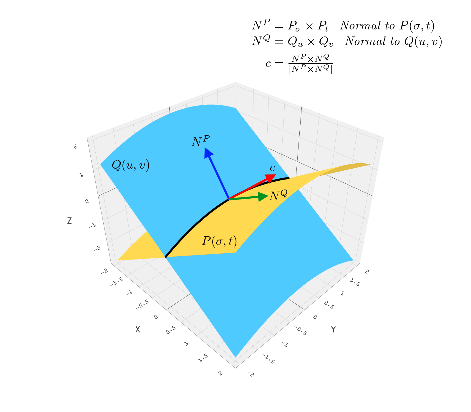
Figure 18: “Marching” an intersection between two NURBS.
There are challenges to note with the non-analytic nature of SSI. Standard methods such as marching methods, have computational limitations and accuracy issues related to the fact that no general algebraic form for the intersection exists. It is a deeper subject, but SSI necessitates algorithms that are approximate.
4.3 The Zoo GPU-Friendly SSI Methodology
4.3.1 Rationale for GPU Acceleration
Traditional SSI methods are CPU based, ie, they are recursive, sequential and conditional. We aim to develop an approach that makes use of the power of modern GPUs. These tend to be brute force with simple instructions and massive data. Benefits of using GPU for SSI, include speed, increased efficiency and handling higher levels of detail.
4.3.2 Patented Algorithm Overview
For the last year or so we have developed an original approach to SSI that is specifically created to leverage a GPU. A patent for this method was recently allowed by the US Patent Office, US patent application No. 18/662056
As mentioned the main idea behind the GPU based method is one of brute force, massive data processed as much as possible in parallel. As seen in Figure 19, the approach is to densely sample both surfaces and compare the resulting point clouds by pairwise point distances, keeping only points that are within a given “tolerance” to each other These points will be close to the SSI. We detail the algorithm in Figures 20 - 22.
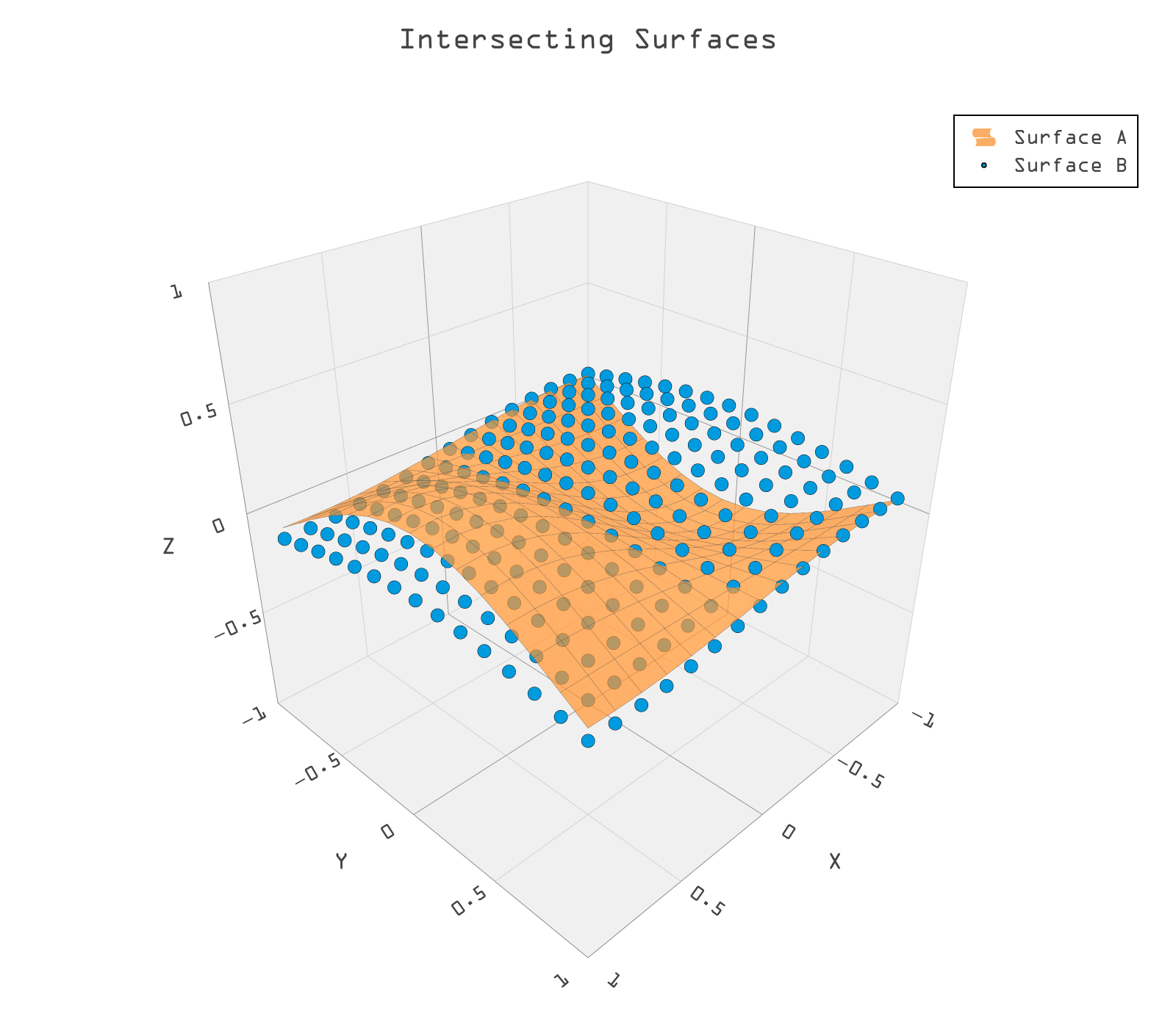
Figure 19: Two intersecting surfaces, one shown as a densely sampled cloud of points.
The sample points are generated as 5 tuples, three xyz object space components, and the two associated uv parameters. Figure 20 below shows two cylindrical surfaces juxtaposed at right angles (left). Each cylinder is sampled at 400 by 400 resolution. The SSI is then approximated by the distance filtered point cloud in object space (right). The cloud spreads out where the intersection curves cross on the cylinders because the surfaces lie closer to each other.
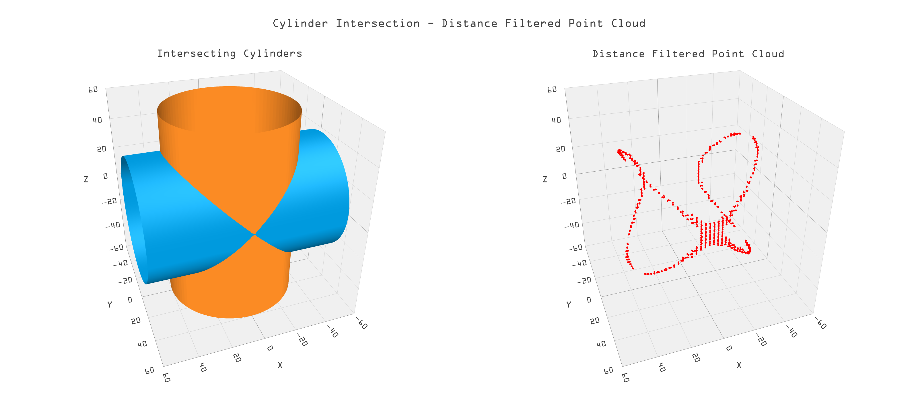
Figure 20: Two cylindrical surfaces and their SSI as points.
If the resolution of the SSI point cloud is too small (as at the SSI cross), one can simply increase the sample size. A more efficient method, however, is to super-sample and compare distances of pairs in smaller, local neighborhoods around the already calculated SSI points, ie, a level of detail approach (LOD). Smaller subpatches created near the SSI points are far fewer in number than the original sample size. Furthermore, the original resolution can be far smaller since it will be refined in the second stage of LOD.
In the figure below the beginning sample size was 40 by 40, producing the red points. The sub-samples were sampled at 20 by 20, giving an effective sampling density of 800 by 800. The subsequent points near the SSI are displayed in blue for an easy to visualize part of the SSI.
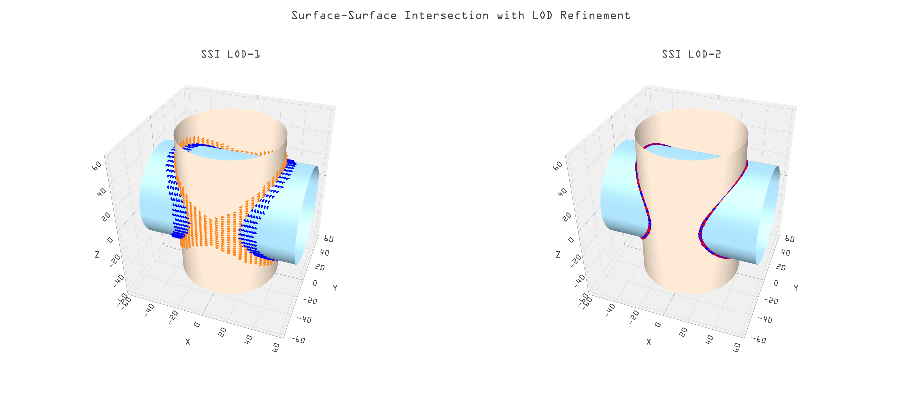
Figure 21: SSI points at two levels of detail for crossed cylinders.
4.3.3 Parameter Space Processing
At this point, we have not really made an intersection curve, rather we have a set of unorganized points, which are close to the intersection. We now focus on the uv components of the points in parameter space to do some advanced processing to improve the quality, precision, and usefulness of the SSI curve that we're going to ultimately produce.
Consider the green surface and gridded surface in Figure 22. The latter is gridded for visibility. This is a more complex intersection than we have yet seen. It will help demonstrate why we need to process in parameter space. Figure 23 shows the corresponding 2d uv points in that space.
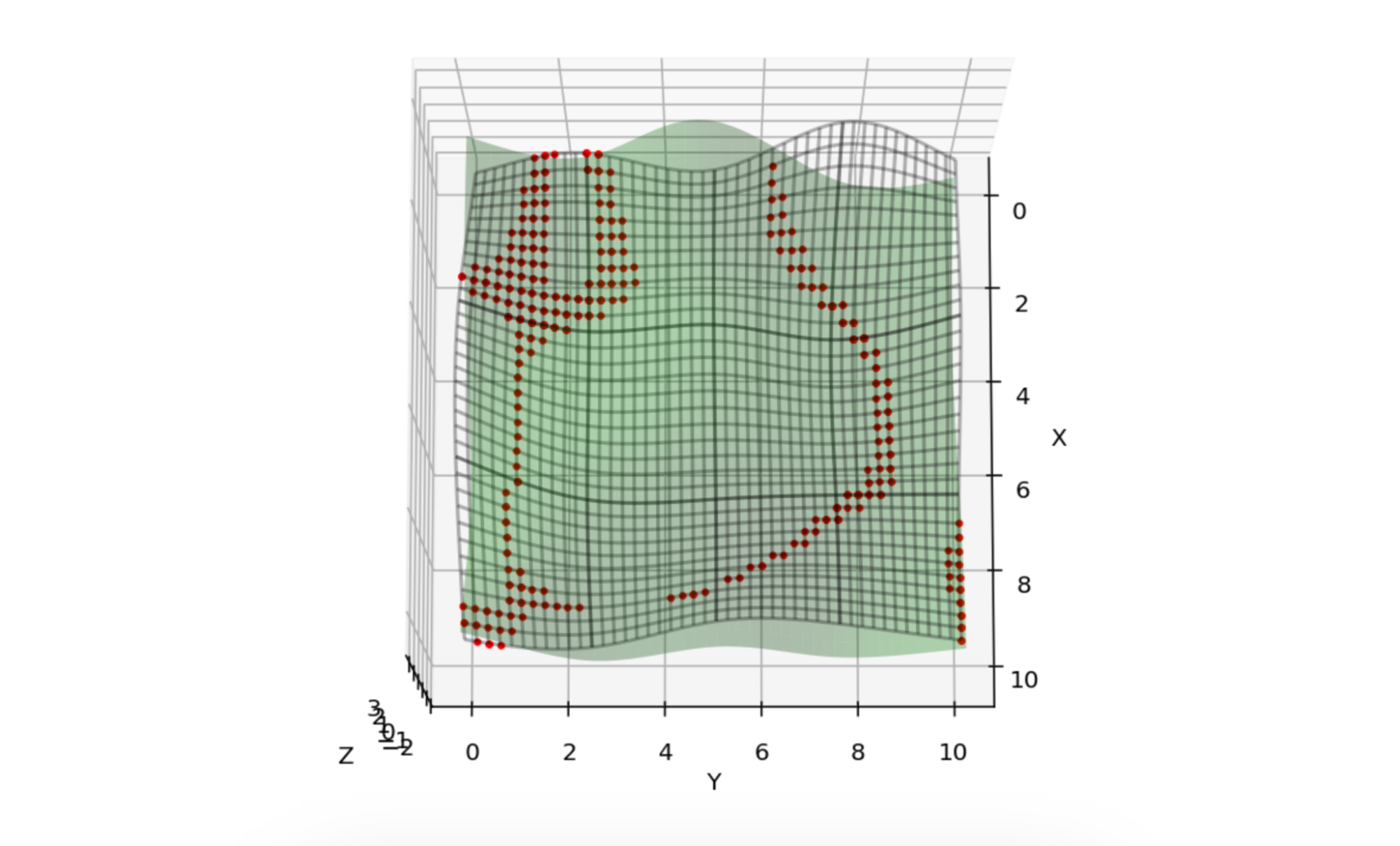
Figure 22: SSI points (red) between green and gridded surfaces.
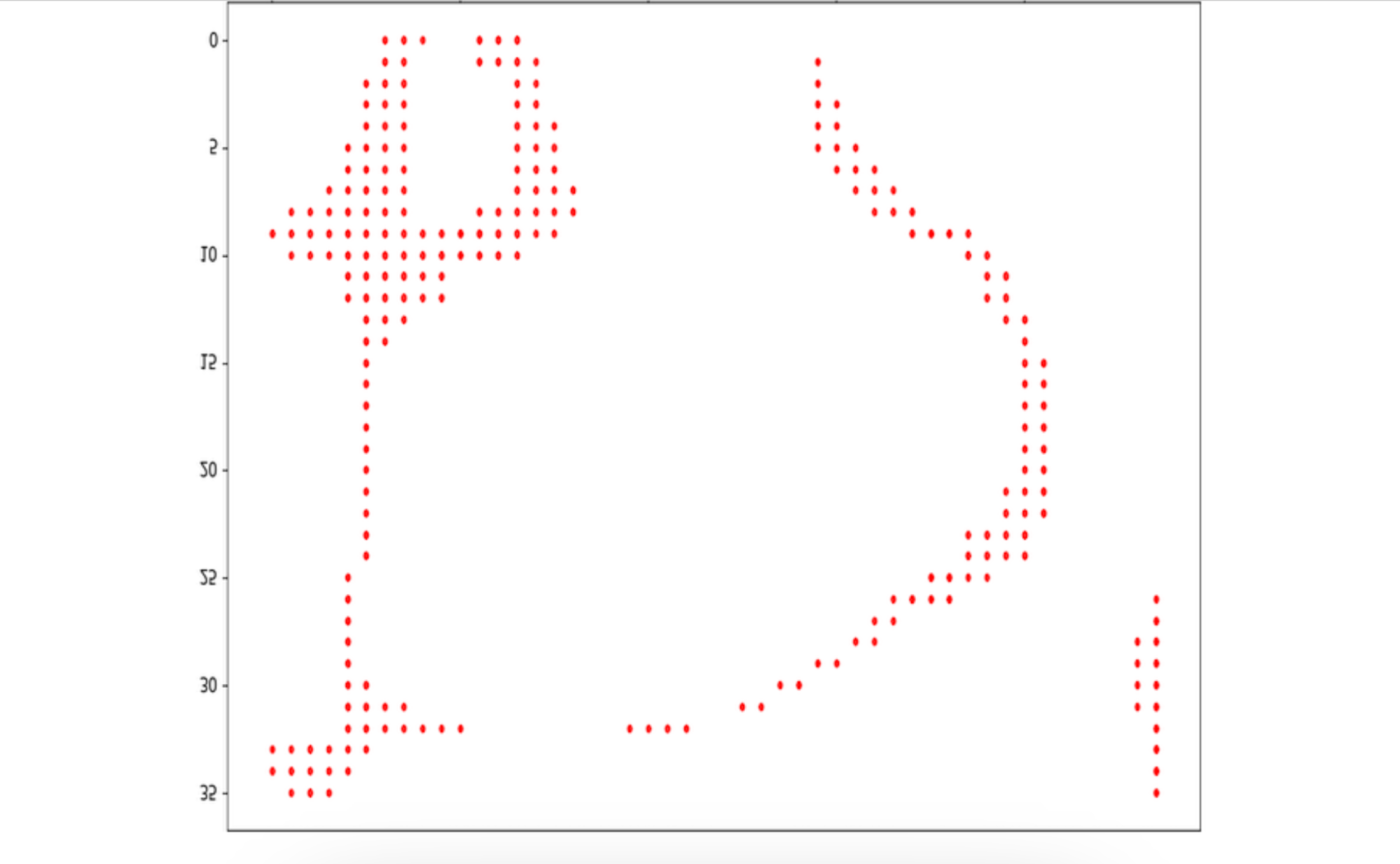
Figure 23: The uv parameter points of the points in Figure 24.
It’s clear from Figure 23 that the thickened areas need to be thinned down to a curve. A number of (image processing) routines exist to do just this such as numpy’s “thinning,” “skeletonize,” or our preferred one, the “medial axis transform” (MAT). Figure 24 is the result of applying MAT to Figure 23.
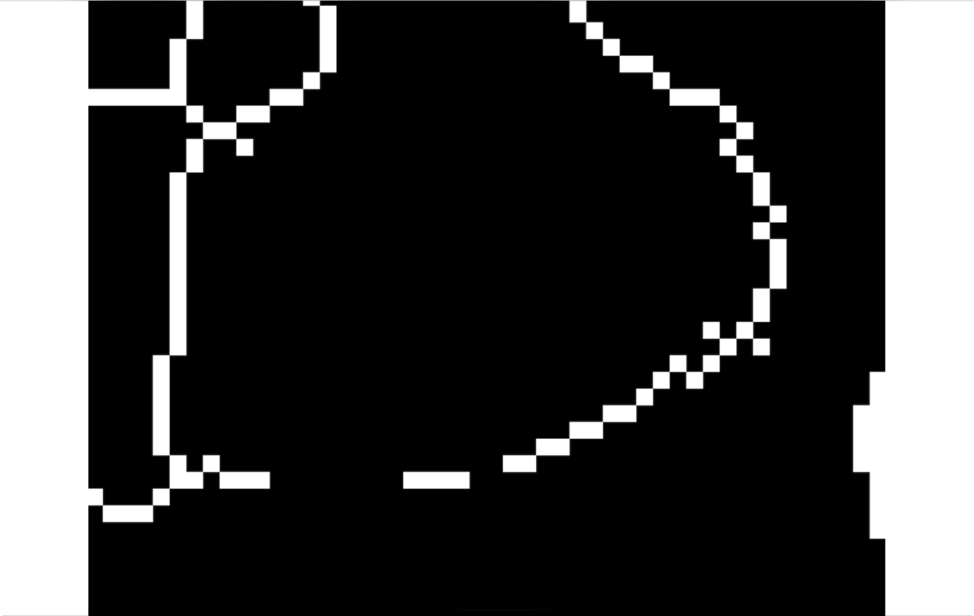
Figure 24: MAT applied to the point set in Figure 23.
Branching
Recall that the point cloud we have been dealing with is an unordered set of points; they do not run nicely from beginning to end. One of our tasks is to order them. They also have different branches as one sees in the above figure. We must also discover the branch points of these as well as end points. Ultimately, we want a simple ordered set of points for each branch. The methods to achieve this goal are succinctly captured in the following python code:
This code creates a distance matrix and a connection-adjacency matrix for a set of points derived
from a binary matrix MATwhich came from the medial axis transform in Figure 24.
The distance matrix dist_mat is based on the squared Euclidean distance between all pairs of
points. An adjacency matrix adj_mat is then created, where a value of 1 indicates that the
distance between two points is less than or equal to 2 (pixels), meaning they are adjacent. It
identifies 'joints' (points with more than 3 neighbors) and 'ends' (points with exactly 2
neighbors).
Hence each point is classified where regular points are marked as 0, joints as 1, ends as 2, and ends on boundaries (at the edges of the defined area) as 3. Figure 25 shows a complex SSI in object space and its corresponding parameter space after the various joints and endpoints have been discovered and categorized.
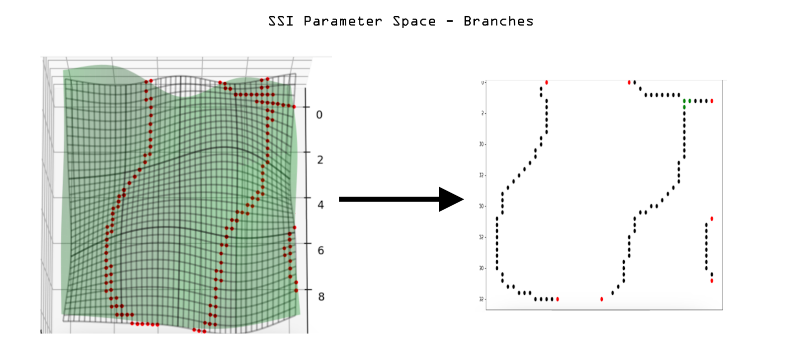
Figure 25: SSI in object space (left) and parameter space uv-points classified by joints (green), end points (red), and simple branch points (black).
4.3.4 Curve Reconstruction and Refinement
Now that the uv-points are divided into simple branches we can begin the final stage of processing, that is, to order the points, convolve them, and create the b-spline curves from them. The convolution and ordering steps can be combined into one. In image processing, convolution is a fundamental operation used for filtering images. It involves applying a filter, also known as a kernel, to an image to perform various tasks such as blurring, sharpening, edge detection, and more. The kernel is a small matrix of numbers, and convolution works by sliding this kernel over the image, calculating the weighted sum of the pixel values covered by the kernel at each position. For example, to apply a Gaussian blur, a Gaussian kernel is convolved with the image, which smooths out rapid changes in pixel intensity. The result of the convolution is a new image that reflects the operations defined by the kernel. Our MAT kernel was chosen to thin out a tracked data set. The next convolution now smooths it. Only now can we consider ordering the points, since the notion of an ordering made no sense on the thick, wiggly set.
We can start at any of the red endpoints we have discovered and then use the adjacency matrix from above method to follow from one point of the branch to the next point, terminating when an endpoint or joint is reached; thus properly ordering each branch.
If we take several points in sequence, instead of just one, and then perform a weighted sum on them as the replacement value, we have essentially done a convolution known as a weighted average that smooths them; thus the convolution becomes an easy extension of the ordering algorithm.
A convolution on an ordered set of points in space is known to have beneficial effects if the points were generated with respect to an underlying ground truth such as SSI:
- It minimizes outliers. Noise is inherent in any approximation as we see that an SSI must be. The discretization of the original surface grids, the inverse mapping to uv space, distance and adjacency matrix calculations can all add noise to the result Convolution tends to remove (a consequence of the central limit theorem in statistics).
- It fills in gaps caused by undersampling. This follows from the weighted averaging.It depends on the weights and size of the kernel.
- It reduces the number of points, keeping the more desirable ones.
- It conditions the points to generate better b-spline curves both by thinning them and ‘straightening’ them out.
All the previous advantages depend on choosing the convolution parameters judiciously. The kernel size and shape affect the value and usability of the final convolved points, that is there is a fair amount of engineering to get the best performance. For any given application there will be specific heuristics to best choose the parameters.
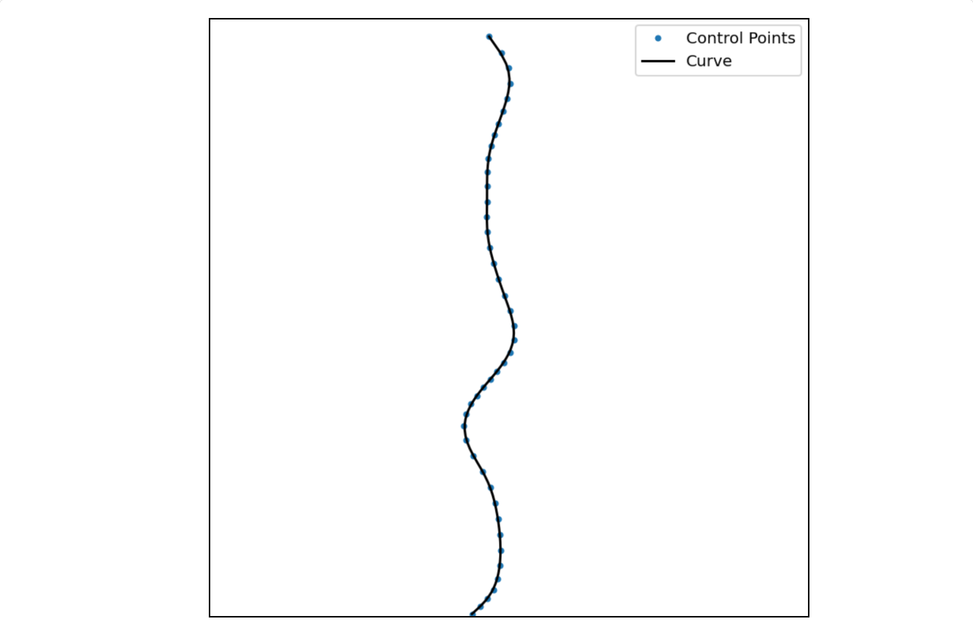
Figure 26: A single branch of uv points which have been convolved with a hat filter, and then fit with a cubic interpolation spline.
Figure 26 represents the final stage of processing in uv-space, which included the mapping from object to parameter space, calculating MAT, distance and adjacency matrices, endpoint and joint discovery, ordering and convolving, and finally, the b-spline fit.
The final stage in our SSI routine is to map the uv branches back to object space by sampling the b-splines and then computing their images in 3d via the user given b-spline functions. Figure 27 shows the mapping of the b-spline in Figure 26 to object space, the red SSI on the top edge.
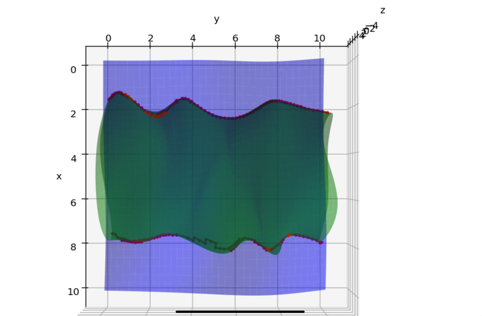
Figure 27. Final step in SSI routine, the red intersection curve on the top.
For someone not familiar with SSI, our routine might seem rather involved. There are several things to note in that regard: First, all high end SSI routines are involved; it is a difficult challenge. In the marching method, for instance, finding joints for branch points is especially troublesome, necessitating analysis of higher order derivatives and repeatedly checking for valid edge loops. Extra effort to find start points and link them to the correct topological pieces is also needed. Second, many of our steps exist to improve the method such as the level of detail for speed, and convolution for accuracy. They are not required. The b-spline fitting benefits downstream operations like trimming and blending.
The SSI routine implicitly assumes that one of the surfaces serves as the master in which parameter space the uv space operations occur, and where the final SSI curve sits. The choice of this surface might depend on features like minimal parameter distortion (as determined by control point distribution) or some flatness criteria.
Another option is to create SSI for each surface and then average the result. This should be even more accurate. Many tests are still needed.
Finally, it should be noted that the performance of our routine depends critically on the sampling of the two surfaces. A separate white paper details the research we have done into the evaluation of NURBS using GPUs.
Figure 28. A good SSI is modest, unassuming, and works!