A Practical Overview of CAD File Formats
- 2.1 Visual Formats
- 2.2 Intermediate formats
- 2.3 Modelling Kernel Formats
- 2.4 Authoring Formats
- 2.5 Tradeoffs
- 2.5.1 Comparison Table
- Footnotes
1 Introduction
This article discusses in brief detail the differences between common CAD formats. The article considers four broad categories of formats: visual, intermediate, modelling kernel, and authoring. The article summarises with a table of the most common formats and their usages.
2 Overview of CAD Formats
2.1 Visual Formats
These kinds of formats are almost exclusively based on polygonal meshes. With enough polygons, and with the observer suitably far away, mesh representations of smooth shapes will indeed appear smooth. This is, however, merely an illusion; zooming in will reveal the faceted surface.
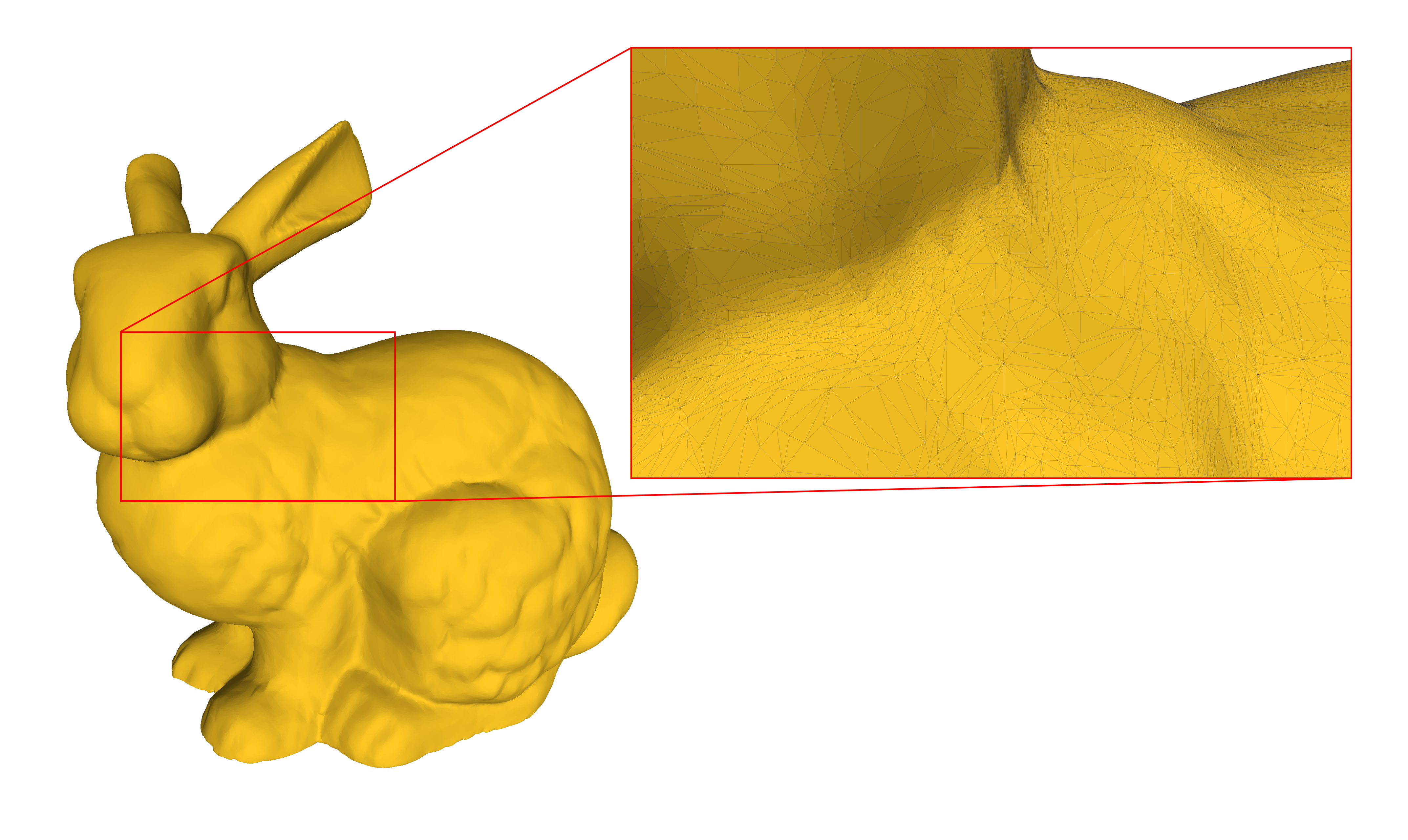
Figure 1: Stanford Bunny With Faceted Surface Highlighting
The most common choice of polygon is the triangle. This is because a triangle sits in a plane unambiguously. The same cannot be said about quadrilaterals since they can have two possible ‘bend’ configurations if their four points do not lie in a plane.
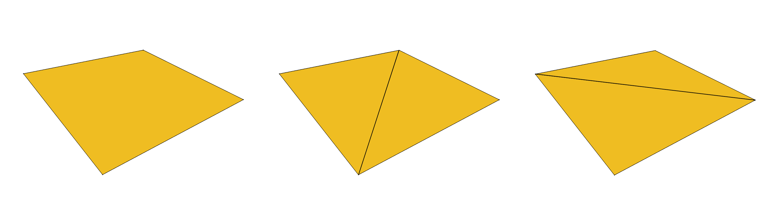
Figure 2: Non-Planar Quadrilateral and Its Two Possible Triangulations
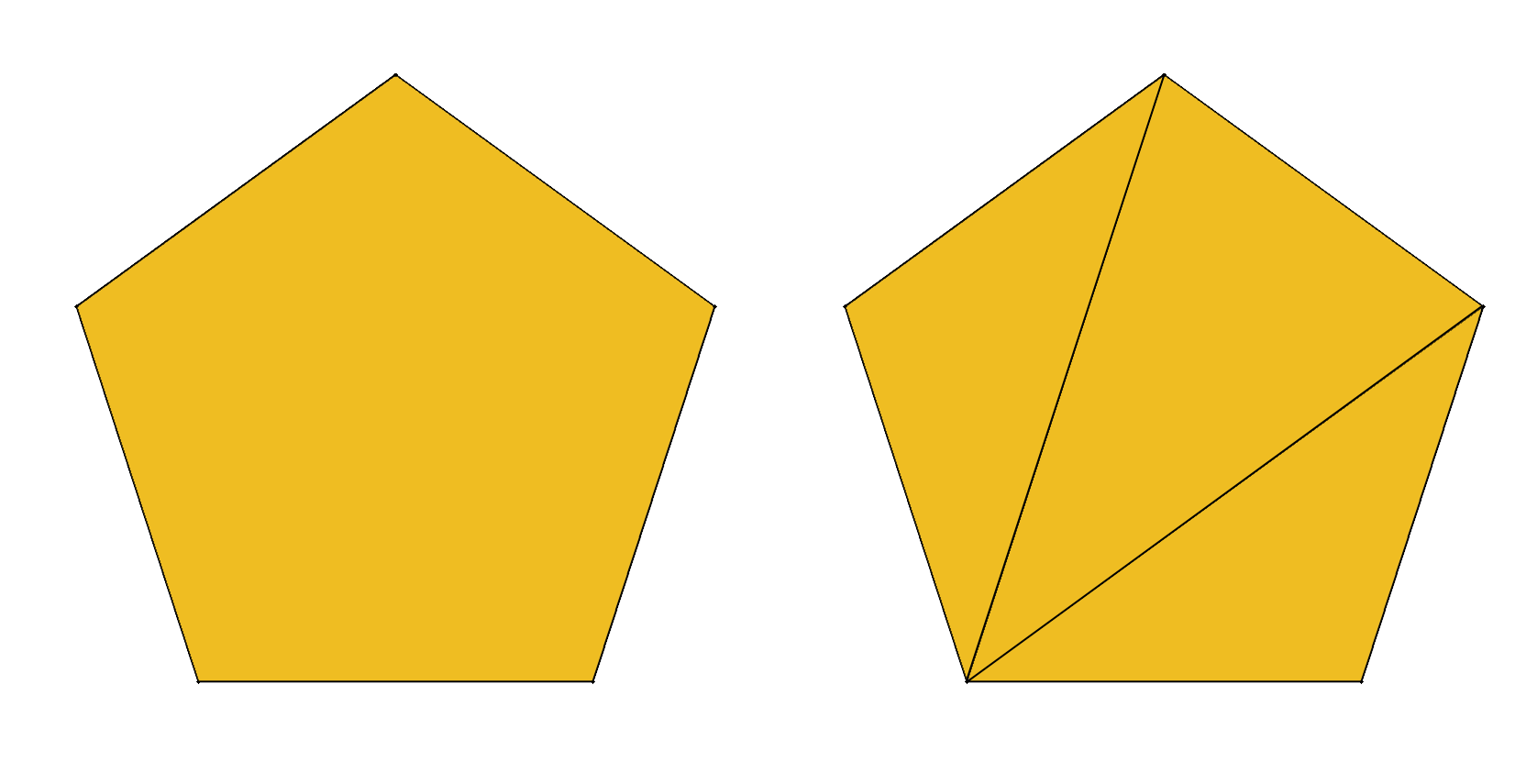
The minimal amount of information required to represent a mesh is an ordered set of points plus a rule to connect them together into polygons. The most common rules are triangle lists, triangle strips, and triangle fans.
The first approach, triangle lists, is often preferred because it maintains a consistent winding order. The winding order is often used in CAD applications to determine whether a polygon is facing toward or away from its observer.
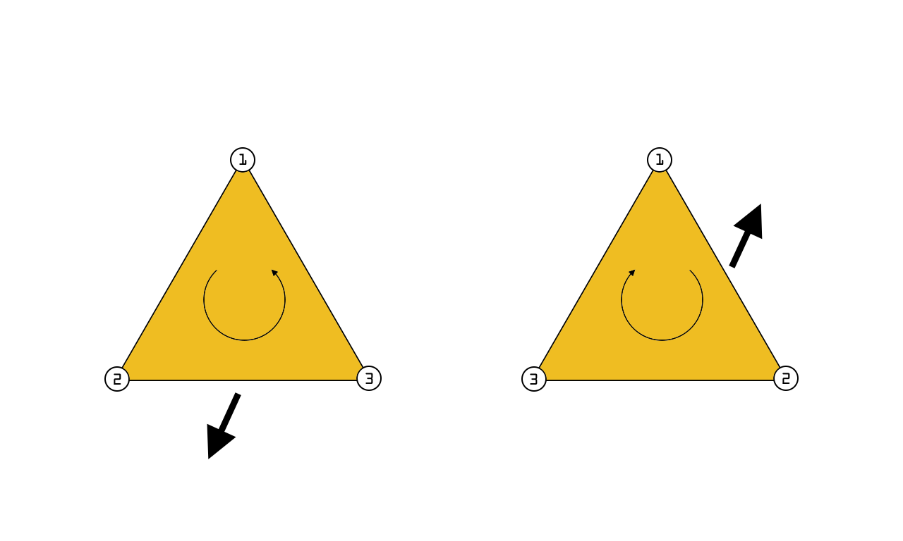
Figure 3: Winding Order of Front-Facing (Left) Versus Rear-Facing (Right) Triangles
Triangle lists are represented in STL as follows:
To avoid duplicating the points (called vertices) in memory, a separate index list is often used to determine the vertex order. This is the approach taken by OBJ, a comparable format. The same two polygons (called faces) are represented in OBJ as follows:
Observe how this format needs only store vertices that are unique. Faces are described by referencing vertices by their index.
For applications such as 3D printing and finite element analysis, knowing only the position of vertices is usually sufficient. In more complex applications, such as game engines, there is often more information contained in a mesh required for rendering. The two most common are explored next: vertex normals and texture coordinates.
On a planar surface, such as a single triangle, the surface normal vector points in the facing direction directly ‘away’ from the surface. The same is also true for non-planar surfaces but its normal vector varies as the surface curves. 3D renderers can use surface normals to compute lighting per-face; however, this draws attention to the model’s facets, removing the illusion of smoothness.
To avoid this problem, 3D renderers compute lighting by considering the average of normal vectors at the vertices. The vertex normals are then interpolated across the planar surface to produce the illusion of smoothness. OBJ allows normals to be specified per vertex whereas STL only allows normals to be specified per facet.
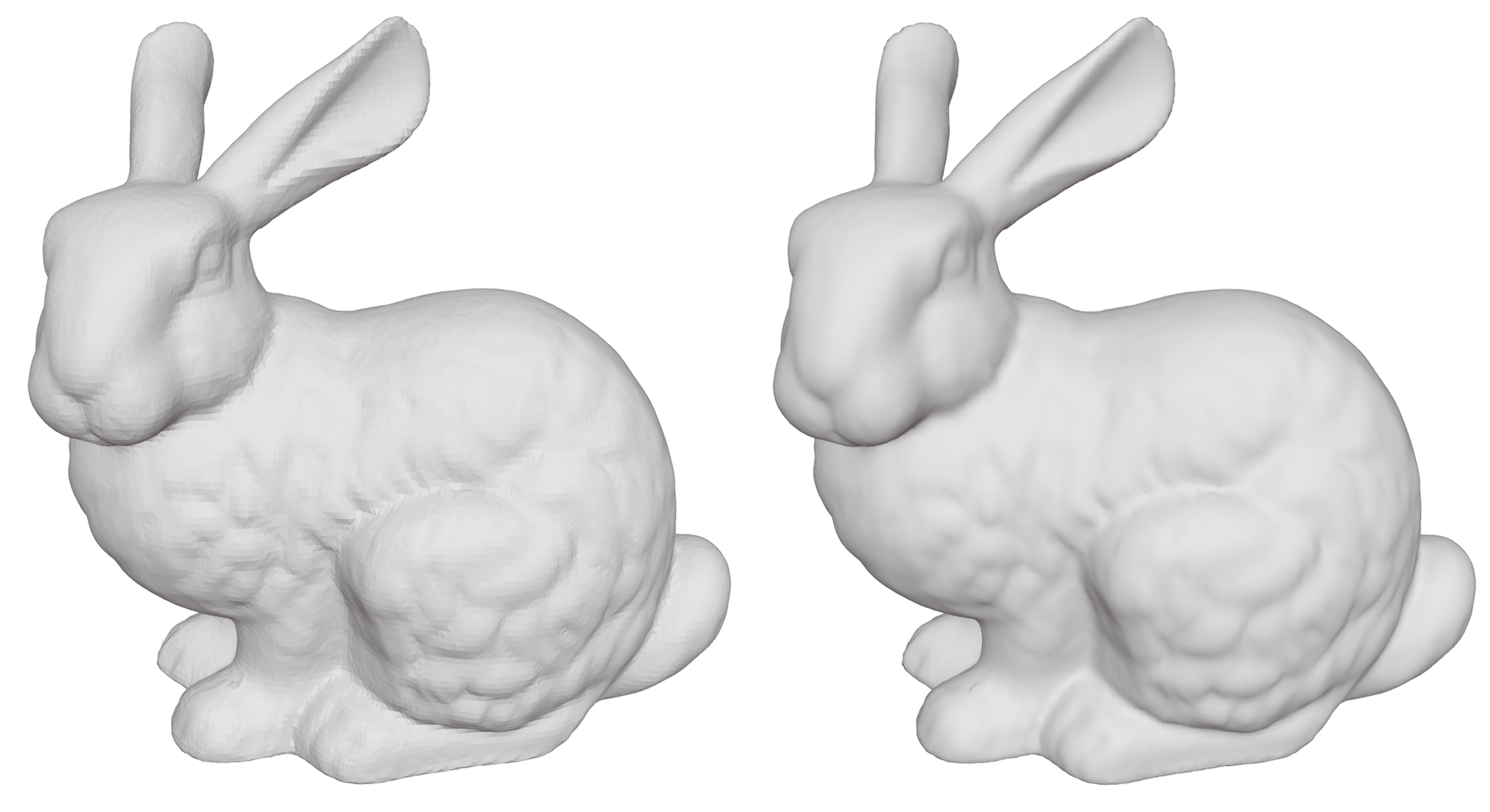
Figure 4: Per-Facet Normals (Left) Versus Averaged Per-Vertex Normals (Right)
The vn element provides vertex normal information in OBJ:
It is common for renderers to ‘paint’ models using an image called a texture. The way this works is the image is given a 2D coordinate space, commonly a unit square, and each 3D vertex coordinate is assigned a corresponding ‘texture coordinate’ in this 2D space. The delicate process of choosing a texture coordinate for each vertex is known as ‘UV unwrapping’ and is typically performed by the model’s creator.
The vt element provides vertex texture coordinates in OBJ:
Thus far, the discussion has focused only on STL and OBJ. These are both plaintext formats, meaning the contents of the file are directly human-readable. This has advantages and disadvantages. One advantage is they can be used with any program that works with text. Another advantage is it is easy for a software engineer to understand and verify its correctness. The main disadvantages of plaintext are the size it occupies in memory and the extra processing time required for a program to write and interpret the data. The alternative to plaintext formats is binary formats1, which instead are directly computer-readable. As these formats are not directly human-readable, a specification must be published to precisely define the layout of the data contained within. Three common binary formats are considered hereafter: binary STL, binary PLY, and glTF.
The binary format of STL is very similar to its plaintext counterpart. There is an 80 byte header (which is nominally empty), followed by the number of triangles, and terminated with the per-triangle vertex data. Each triangle requires 50 bytes of storage. In comparison, a single character in the plaintext format occupies a single byte. The previous STL example, without facet normals, with no decimal places, and with whitespace removed, occupied 188 bytes. The same data with facet normals would occupy a mere 100 bytes in binary STL.
The plaintext and binary PLY formats are also similar to each other. PLY was designed with more flexibility in mind in terms of what data can be stored. Whereas STL and OBJ have a pre-determined set of data that can be described, the data in a PLY file is self-described by its header (which is human-readable); the most important data items being reserved and formalised in the specification. Below is the STL example expressed as a plaintext PLY file. Beyond the header, the plaintext data is converted to binary trivially based on the self-described property sizes.
The increased flexibility of PLY allows for extensibility and arbitrary user data, at the expense of being slightly more complicated for importers to process. For example, the number of vertices per face (essentially, the type of polygon) is variable and therefore unpredictable. It is common for importers to split polygons with more than three vertices into multiple triangles.
The naming and ordering of elements and properties is also variable. For example, use of the
property name vertex_index in place of vertex_indices is not uncommon.
glTF is a relatively new format which has a hybrid plaintext and binary structure. The plaintext
half is encoded in JavaScript Object Notation (JSON), itself an ubiquitous storage format, to store
a rich set of user data. The binary half is optional; where provided, its contents are described in
the plaintext half. The format extends beyond mere polygons, facilitating storage of animated scenes
and data for photorealistic rendering techniques.
glTF offers substantially more flexibility than its historical counterparts but at the expense of verbosity. The following section walks through the glTF version of the STL example described earlier.
The glTF version is identified under the asset property. This is the only required part of the format. A single scene is (optionally) defined as the default choice; this scene is then defined as a composition of nodes, which may reference other nodes to form a tree; and the sole node in the scene instantiates a renderable mesh.
Similar to PLY, the data contained in a polygonal mesh and its layout is variable. These properties are called vertex ‘attributes’ in glTF terminology. The location, size, and layout of the corresponding attribute data is then described using ‘accessors’ into ‘buffer views’ and buffer views into data buffers.
glTF has three modes of storage for its buffer data: it may be included within the JSON, using ‘base64’ encoding, provided as a separate binary file (as demonstrated above), or bundled in the same file using the binary glTF (GLB) mode. The GLB mode has an extra small header before the JSON portion to identify itself as such.
2.2 Intermediate formats
An important concept underpinning many CAD applications is the idea of a spline surface. A spline surface uses familiar vertices as before but, instead of joining them into polygons, a rule for interpolating between the points is defined.
One of the most common and general forms of spline surfaces is known by the acronym NURBS. The precise definition is technical in nature and irrelevant to this topic; what is relevant is they are able to represent many kinds of surfaces exactly, including spheres, cones, and ellipsoids.
The familiar OBJ format provides a limited way of defining NURBS surfaces. Here is one such example, demonstrating an open cylinder:
It is possible to represent solids as a composition of spline surfaces. Doing so however introduces ambiguity where the surface joins since it is not possible to match exactly in general. IGES is an example of an intermediate format which had this issue for most of its history.
To remedy the ambiguity problem, boundary curves are used to explicitly define where surfaces should join. This combination of surfaces and boundary curves is often referred to as boundary representation2, or ‘B-rep’ for short.
B-reps, by necessity, also carry topological information describing the relationship between each surface. In B-rep terminology, bounded surfaces are called ‘faces’, boundary curves correspond to ‘edges’, and the edges join at the familiar vertices. Note that the vertices themselves are distinct coordinates resolving the ambiguity problem of multiple edges meeting at a common point.
STEP is an example of an intermediate format which is able to carry B-rep data, amongst other kinds of data such as geometric dimensioning and tolerancing information. IGES gained topological information as part of its fifth version release in 1991 but has since been superseded largely by STEP.
A solid object (a manifold3 in B-rep terminology) is a collection of faces which combine such that there is a distinct ‘outside’ and ‘inside’ volume.
Surfaces, curves, vertices, faces, etc., are all deemed ‘entities’ and are each assigned a unique ID number. Entities can, and often do, reference other entities. References can be made to entities before they are defined.
The vertex_point entity represents vertices. A vertex is a topological construct in STEP and must be linked to a geometric construct. In this example, the vertex point is linked to a Cartesian point in 3D space.
Edges are typically represented using the edge_curve entity. Edges are linked to a geometric curve in 3D space.
The final .T. value (which means true) expresses whether the direction of the curve matches that of the edge endpoints.
Curves are defined in various ways. A common kind of curve, a circle, is expressed as:
If it isn’t already clear, STEP (or, more precisely, the EXPRESS exchange format) is highly verbose. Its extensive number of entities make it a double-edged sword, being versatile but complex to process for a CAD application.
This complexity means that different applications may treat STEP files slightly differently to each other. For example, one CAD program might not support a particular STEP entity, or handle an uncommon entity incorrectly.
A typical data hierarchy for a B-rep model in a STEP file is as follows:
Common curve entities include:
b_spline_surfaceconical_surfacecylindrical_surfaceplanespherical_surfacetoroidal_surface
Common surface entities include:
b_spline_curvecirclelinesurface_curve
Zoo is developing an extension to glTF that allows for solids to be described as polygonal meshes and parametric boundary representations mutually. This combines the benefits of each representation and reduces the need for complex and time-consuming conversion steps. In comparison to STEP, the extension continues to be encoded as plaintext as part of the JSON portion but is substantially less verbose. The following section walks through an excerpt of a glTF file describing a solid cylinder using Zoo’s KITTYCAD_boundary_representation extension.
The majority of the B-rep data extends the root JSON object. A set of solids are defined in terms of ‘shells’; the former is referenced within the glTF scene hierarchy and the latter references other objects within the extension’s own data hierarchy.
Above, a solid is defined in terms of a single shell in its ‘same’ sense. With the exception of vertices, all objects have two orientations which are referred to as same-sense and reverse-sense. A specific orientation is selected using ±1 in addition to the index of the referenced item.
Shells are composed of connected faces, faces are defined on parametric surfaces bounded by 3D loops, and loops are composed of connected edges.
Edges are defined by parametric curves in 3D space and join at vertices. B-rep vertices are distinct from mesh vertices, defined by only their position in 3D space.
2.3 Modelling Kernel Formats
The collection of algorithms used to compute the geometry for computer aided designs form what is known as the modelling kernel. This is a fundamental component of CAD/CAM software and it is often reused between the suites of different vendors. For example, both SOLIDWORKS and NX use the Parasolid modelling kernel; AutoCAD and Inventor both use the ShapeManager kernel. Some programs such as Rhino3D and CATIA use their own kernel. Zoo is developing its own GPU accelerated modelling kernel which can be read more about here.
Modelling kernel formats typically do not offer any more information than comparable intermediate formats; however, their benefit over comparable formats is that their representation matches the kernel exactly. As a contrived example, an intermediate format might represent a circular arc using an angle whereas a modelling kernel might represent a circular arc as three points; these kinds of differences introduce potential problems as one representation needs to be converted into another.
2.4 Authoring Formats
This category describes all formats specific to a particular application, for example, a SOLIDWORKS part file. These formats are generally proprietary and usually closed, so examples cannot be provided here. Additionally, measures are sometimes taken to obfuscate the contents of authoring files to discourage reverse engineering by other companies. Authoring formats are usually binary encoded and sometimes compressed or even encrypted.
2.5 Tradeoffs
Like many things in life, choices are seldom black-and-white but rather present tradeoffs between desirable and undesirable qualities. The choice for which format should be chosen will depend on what is needed from the export.
Requirements a user might consider from an export could include:
- Precision of data exchange
- Ability to modify exchanged models
- Software compatibility
- Protection of intellectual property
- Speed of data exchange
The introduction described four broad categories of formats: visual, intermediate, modelling kernel, and authoring. This categorisation produces a hierarchy of detail, where each format contains more information than the previous. An analogy of a work of fine art is presented to demonstrate:
Authoring files are the original artwork. Sharing the authoring file guarantees precision and modifiability at the expense of software compatibility and protection of intellectual property. In this category are found formats from SOLIDWORKS, CATIA, Inventor, Creo, etc.
Modelling kernel formats are akin to a close like-for-like reproduction of the original. The data exchange is likely to be as precise as the original, less risky than sending the original, but it may be less convenient to modify. Software compatibility may still be an issue. In this category are found formats from ACIS, Parasolid, Rhino 3D, etc.
Intermediate formats are akin to a mass-produced print of the original. Much of the original details such as features are lost but precision still remains in the B-rep representation. The most notable formats in this category are STEP, IGES, and glTF when combined with Zoo’s KITTYCAD_boundary_representation extension.
Visual formats are akin to a sketch of the original. Almost all of the details are lost. Popular formats include glTF, STL, PLY, OBJ, and FBX.
2.5.1 Comparison Table
| Extensions | Description | Category | Open | Mesh | B-rep | Text | Binary |
|---|---|---|---|---|---|---|---|
obj, mtl | Wavefront Object | Visual | Y | Y | [1] | Y | N |
gltf, glb | Khronos OpenGL Transmission | Visual | Y | Y | [2] | Y (gltf) | Y (glb) |
sldprt, sldasm | SOLIDWORKS Part/Assembly | Authoring | N | N | Y | ||
catpart, catproduct | CATIA Part/Product | Authoring | N | N | Y | ||
step, stp | ISO 10303-21 Standard for the Exchange of Product Model Data | Intermediate | Y | Y | Y | Y | N |
x_t, x_b | Parasolid XT | Kernel | Y | Y | Y | Y (x_t) | Y (x_b) |
sab, sat | ACIS-SAT | Kernel | N | Y (sat) | Y (sab) | ||
stl | Stereolithography | Visual | Y | Y | N | Y | Y |
ply | Stanford Polygon | Visual | Y | Y | N | Y | Y |
fbx | Autodesk Filmbox | Visual | Y | Y | N | Y | Y |
pdf, prc | ISO 14739-1 Portable Document | Intermediate | Y | Y | Y | N | Y |
dae | Khronos COLLADA | Visual | Y | Y | N | Y | N |
dwg | AutoCAD | Authoring | Y | Y | Y | N | Y |
prt [4], asm | Creo Part/Assembly | Authoring | N | N | Y | ||
jt | ISO 14306 Jupiter Tessellation | Intermediate | Y | Y | Y | N | Y |
ipt, aim | Inventor Part/Assembly | Authoring | N | N | Y | ||
3mf | 3D Manufacturing | Visual | Y | Y | N | Y | N |
3dm | Rhino 3D Model | Kernel | Y | Y | Y | N | Y |
iges, igs | ASME Y14.26M Initial Graphics Exchange Specification | Intermediate | Y | N | [3] | Y | N |
prt [4] | NX Part | Authoring | N | N | Y |
Table Notes
- NURBS surfaces are available without topology but this is rarely used.
- B-reps available with KITTYCAD_boundary_representation subject to software support.
- Surfaces are available without topology.
- Creo and NX part files share the same file extension.
Footnotes
Footnotes
-
Compressing (‘zipping’) a plaintext file will reduce its size but not necessarily its processing time. ↩
-
A boundary representation is technically any representation that distinguishes ‘inside’ from ‘outside’ areas, which would include polygonal meshes, but the term ‘B-rep’ is understood colloquially to refer to the noted form specifically. ↩
-
Non-manifold B-reps are beyond the scope of this page. Nonetheless, for the curious reader, Klein bottles and Möbius strips are examples of non-manifold solids and surfaces respectively. ↩